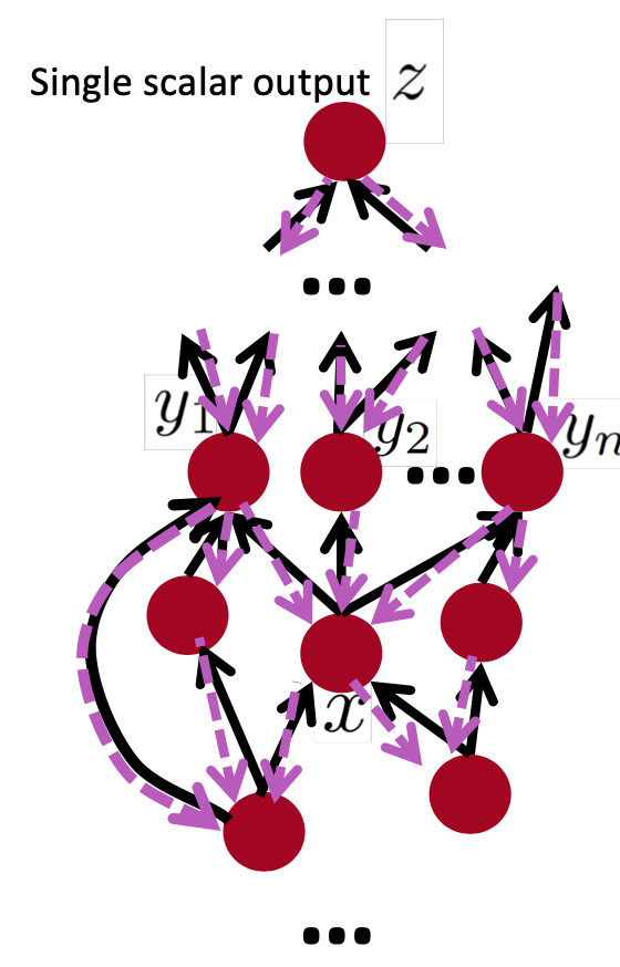
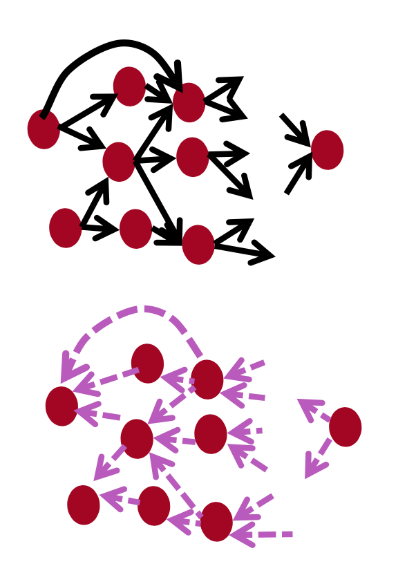
General Computation Graph
- Fprop: visit nodes in topological sort order
- Compute value of node given predecessors
- Bprop:
- initialize output gradient = 1
- visit nodes in reverse order:
- Compute gradient wrt each node using gradient wrt successors \[{y_1,y_2, \cdots, y_n} = successors of x\] \[\frac{\partial z}{\partial x} = \sum_{i=1}^{n}\frac{\partial z}{\partial y_i}\frac{\partial y_i}{\partial x}\] Done correctly, big O() complexity of fprop and bprop is the same
Automatic Differentiation
- The gradient computation canbe automatically inferred from the symbolic expression of the fprop
- Each node type needs to know how to compute its output and how to compute the gradient wrt its inputs given the gradient wrt its output
- Modern DL frameworks(Tensorflow, PyTorch, etc.) do backpropagation for you but mainly leave layer/node writer to hand-calculate the local derivative
Example: Sigmoid
The gates we introduced above are relatively arbitrary. Any kind of differentiable function can act as a gate, and we can group multiple gates into a single gate, or decompose a function into multiple gates whenever it is convenient. Lets look at another expression that illustrates this point:
\[f(w,x) = \frac{1}{1+e^{-(w_0x_0 + w_1x_1 + w_2)}}\]
We have the knowlege of derivatives
\[\begin{aligned} f(x) = \frac{1}{x} \hspace{1in} & \rightarrow \hspace{1in} \frac{df}{dx} = -1/x^2 \\ f_c(x) = c + x\hspace{1in} & \rightarrow \hspace{1in} \frac{df}{dx} = 1 \\ f(x) = e^x\hspace{1in} & \rightarrow \hspace{1in} \frac{df}{dx} = e^x \\ f_a(x) = ax\hspace{1in} & \rightarrow \hspace{1in} \frac{df}{dx} = a \\ \end{aligned}\]
the picture blow shows the visual representation of the computation. The forward pass computes values from inputs to output (shown in green). The backward pass then performs backpropagation which starts at the end and recursively applies the chain rule to compute the gradients (shown in red) all the way to the inputs of the circuit. The gradients can be thought of as flowing backwards through the circuit.
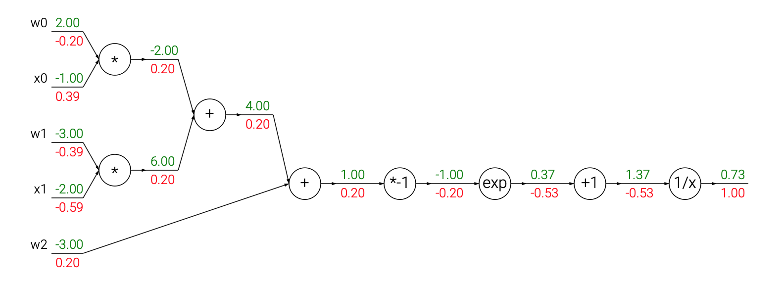
It turns out that the derivative of the sigmoid function with respect to its input simplifies if you perform the derivation (after a fun tricky part where we add and subtract a 1 in the numerator):
\[\sigma(x) = \frac{1}{1+e^{-x}} \\\\ \rightarrow \hspace{0.3in} \frac{d\sigma(x)}{dx} = \frac{e^{-x}}{(1+e^{-x})^2} = \left( \frac{1 + e^{-x} - 1}{1 + e^{-x}} \right) \left( \frac{1}{1+e^{-x}} \right) = \left( 1 - \sigma(x) \right) \sigma(x)\]
As we see, the gradient turns out to simplify and becomes surprisingly simple. For example, the sigmoid expression receives the input 1.0 and computes the output 0.73 during the forward pass. The derivation above shows that the local gradient would simply be (1 - 0.73) * 0.73 = 0.2, as the circuit computed before (see the image above), except this way it would be done with a single, simple and efficient expression (and with less numerical issues). Therefore, in any real practical application it would be very useful to group these operations into a single gate. Lets see the backprop for this neuron in code:
1 | w = [2,-3,-3] # assume some random weights and data |
Staged computation
Lets see this with another example. Suppose that we have a function of the form:
\[f(x,y) = \frac{x + \sigma(y)}{\sigma(x) + (x+y)^2}\]
We don’t need to have an explicit function written down that evaluates the gradient. We only have to know how to compute it. Here is how we would structure the forward pass of such expression:
1 | x = 3 # example values |
Computing the backprop pass is easy: We’ll go backwards and for every variable along the way in the forward pass (sigy, num, sigx, xpy, xpysqr, den, invden) we will have the same variable, but one that begins with a d, which will hold the gradient of the output of the circuit with respect to that variable.
1 | # backprop f = num * invden |
Patterns
- add distributes the upstream gradient: The add gate always takes the gradient on its output and distributes it equally to all of its inputs, regardless of what their values were during the forward pass. This follows from the fact that the local gradient for the add operation is simply +1.0, so the gradients on all inputs will exactly equal the gradients on the output because it will be multiplied by x1.0 (and remain unchanged).
- max “routes” the upstream gradient: The max gate routes the gradient. Unlike the add gate which distributed the gradient unchanged to all its inputs, the max gate distributes the gradient (unchanged) to exactly one of its inputs (the input that had the highest value during the forward pass). This is because the local gradient for a max gate is 1.0 for the highest value, and 0.0 for all other values.
- mul switches the upstream gradient: The multiply gate is a little less easy to interpret. Its local gradients are the input values (except switched), and this is multiplied by the gradient on its output during the chain rule.
Implementation
1 | class MultiplyGate: |
Reference
- lecture notes and slides from http://cs231n.github.io/optimization-2/
- lecture notes and slides from http://web.stanford.edu/class/cs224n/