0%

Fourier Transform

Fourier Transform

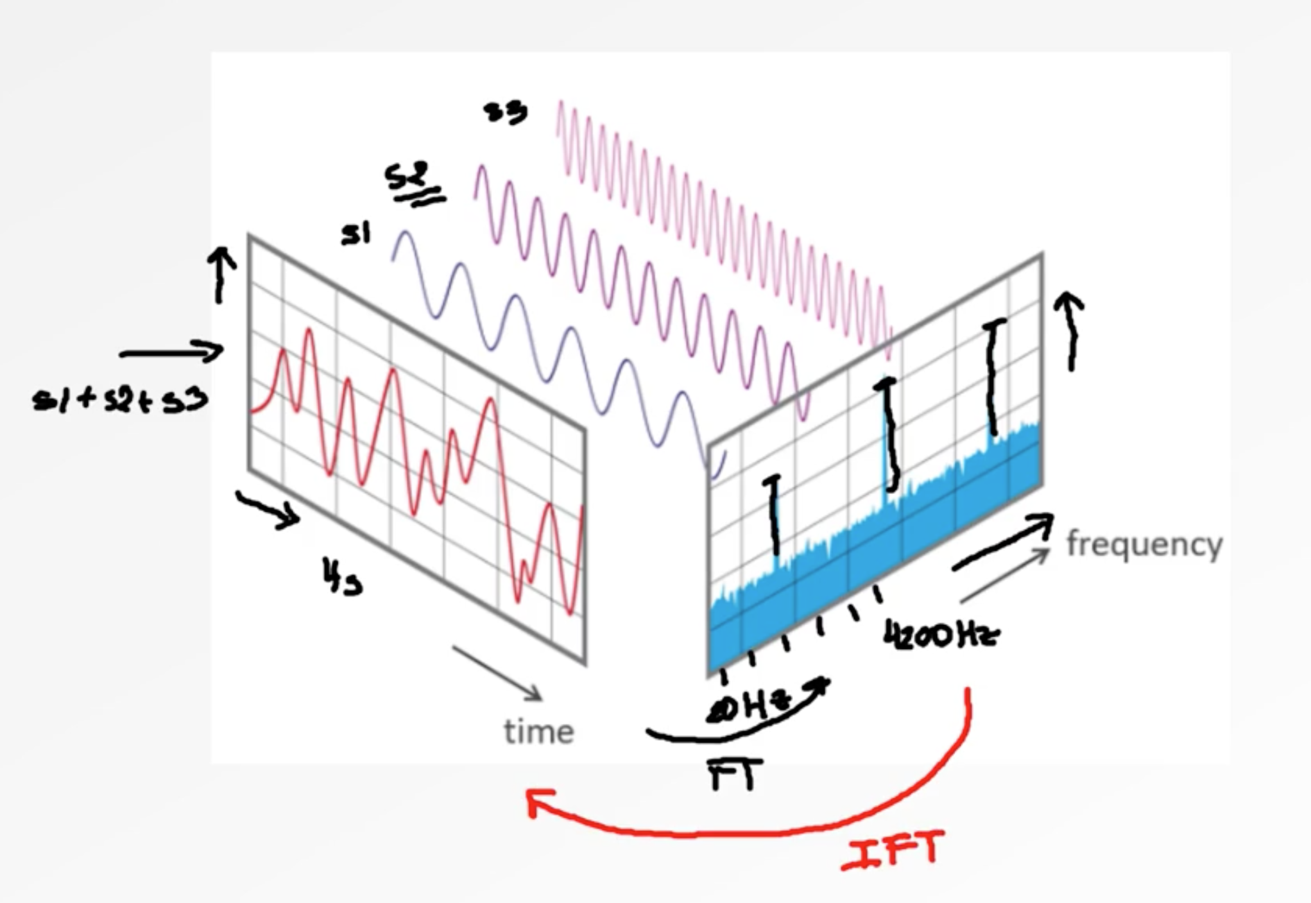
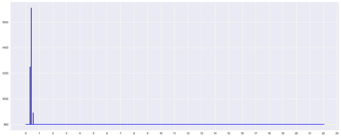
The Fourier transform (FT) decomposes a function (often a function of time, or a signal) into its constituent frequencies.

One motivation for the Fourier transform comes from the study of Fourier series. In the study of Fourier series, complicated but periodic functions are written as the sum of simple waves mathematically represented by sines and cosines. The Fourier transform is an extension of the Fourier series that results when the period of the represented function is lengthened and allowed to approach infinity.

The Fourier transform of a function f is traditionally denoted \(\hat{f}\), by adding a circumflex to the symbol of the function. There are several common conventions for defining the Fourier transform of an integrable function

\[\hat{f}(\xi) = \int_{-\infty}^{\infty} f(x)\ e^{-2\pi i x \xi}\,dx\]

If we want to describe a signal, we need three things : - The frequency of the signal which shows, how many occurrences in the period we have. - Amplitude which shows the height of the signal or in other terms the strength of the signal. - Phase shift as to where does the signal starts.

1
2
3
4
5
6
7
8
9
10
11
12
13
14
15
16
17
18
19
20
21
22
23
24
25
26
27
28
29
30
31
32
33
34
35
36
37
38
39
40
41
42
43
44
45
46
47
48
import numpy as np

import matplotlib.pyplot as plt

import math

from numpy.fft import fft


def gen_wave (freq, amp, T, sr):

time = np.arange(0,T,1/sr)

X = amp*np.sin(2*np.pi*freq*time)

return time,X


plt.style.use("seaborn")
plt.rcParams["xtick.labelsize"] = 14
plt.rcParams["ytick.labelsize"] = 14

f, axarr = plt.subplots(2, figsize=(20, 8))

sr=50 #in Hz

x,y = gen_wave(3,2,1,sr)
x,y2 = gen_wave(5,3,1,sr)

y = y + y2

axarr[0].plot(x, y)

n = len(y)
p = fft(y) # take the fourier transform

mag = np.sqrt(p.real**2 + p.imag**2)

mag = mag * 2 / n

mag = mag[0:math.ceil((n)/2.0)]

x = np.arange(0, len(mag), 1.0) * (sr / n)

axarr[1].bar(x, mag, color='b')
axarr[1].xaxis.set_ticks(np.arange(min(x), max(x)+1, 1.0))

plt.show()
png

Decompose the cord

A special case is the expression of a musical chord in terms of the volumes and frequencies of its constituent notes.

1
2
3
4
5
6
7
8
9
10
11
12
13
14
15
16
17
18
19
20
21
22
23
24
25
26
27
28
29
30
31
32
"""
(C) 2018 Nikolay Manchev

This work is licensed under the Creative Commons Attribution 4.0 International
License. To view a copy of this license, visit http://creativecommons.org/licenses/by/4.0/.
"""

import numpy as np

import matplotlib.pyplot as plt

from scipy.io import wavfile

fs, snd = wavfile.read("output.wav")

snd = snd / (2.**15)
s1 = snd[:,0]

plt.figure(figsize=(20, 8))
plt.style.use("seaborn")

time = np.arange(0, s1.shape[0], 1)
time = (time / fs) * 1000

plt.plot(time, s1, color='b')

plt.ylabel('Amplitude', fontsize=16)
plt.xlabel('Time (ms)', fontsize=16)
plt.xticks(fontsize=14)
plt.yticks(fontsize=14)

plt.show()
png
1
2
3
4
5
6
7
8
9
10
11
12
13
14
15
16
17
18
19
20
21
22
23
24
25
26
27
28
29
30
31
32
33
34
35
36
37
38
39
40
41
42
43
44
45
46
47
48
49
"""
(C) 2018 Nikolay Manchev

This work is licensed under the Creative Commons Attribution 4.0 International
License. To view a copy of this license, visit http://creativecommons.org/licenses/by/4.0/.
"""


import numpy as np

import matplotlib.pyplot as plt

import math

from scipy.io import wavfile

from numpy.fft import fft

plt.rcParams["xtick.labelsize"] = 14
plt.rcParams["ytick.labelsize"] = 14
plt.style.use("seaborn")

threshold = 800
fs, snd = wavfile.read("output.wav")
y = snd[:,0]

plt.figure(figsize=(20, 8))

n = len(y)
p = fft(y)

mag = np.sqrt(p.real**2 + p.imag**2)

mag = mag * 2 / n

mag = mag[0:math.ceil((n)/2.0)]

freq = np.arange(0, len(mag), 1.0) * (fs / n)

if threshold != 0:
print(np.unique(np.rint(freq[np.in1d(mag, mag[mag>threshold])])))
mag[mag<threshold]=threshold

plt.plot(freq/1000, mag, color='b')
plt.xticks(np.arange(min(freq/1000), max(freq/1000)+1, 1.0))

plt.show()


[329. 330. 415. 555.]
png

Wavelet transform

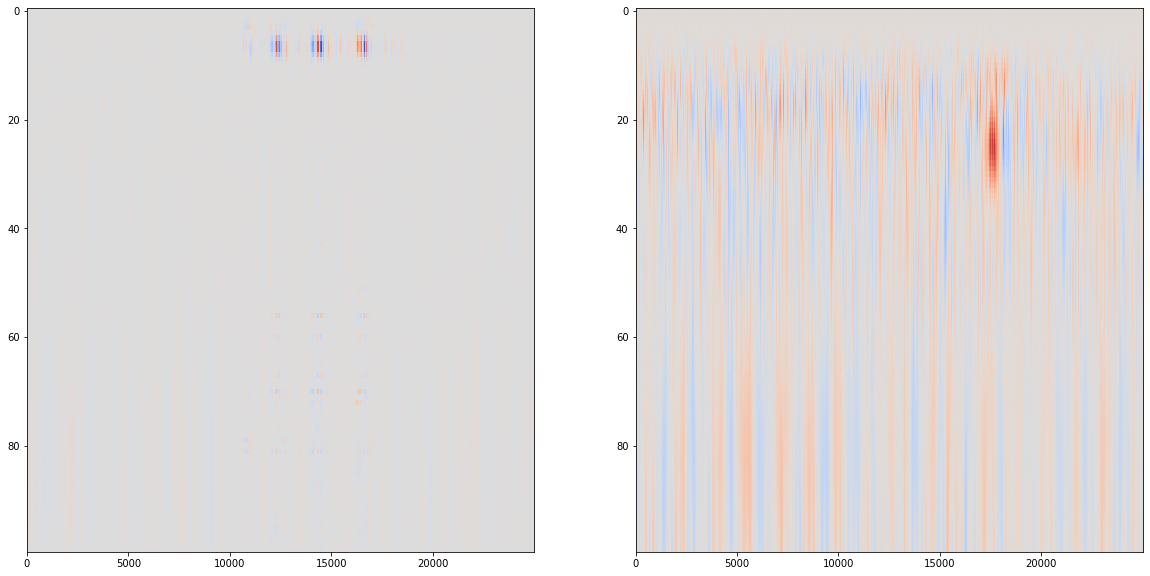
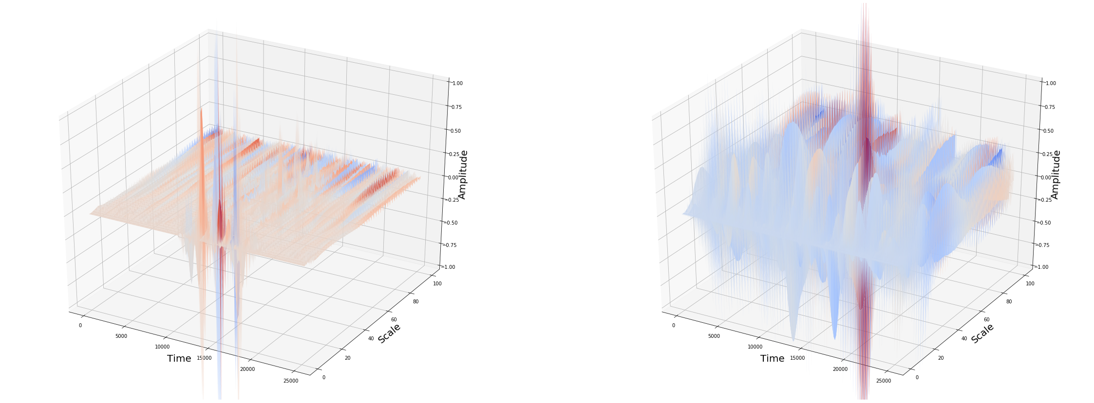
Wavelets have some slight benefits over Fourier transforms in reducing computations when examining specific frequencies. However, they are rarely more sensitive, and indeed, the common Morlet wavelet is mathematically identical to a short-time Fourier transform using a Gaussian window function. The exception is when searching for signals of a known, non-sinusoidal shape (e.g., heartbeats); in that case, using matched wavelets can outperform standard STFT/Morlet analyses.

\[X(a,b) = \frac{1}{\sqrt{a}}\int_{-\infty}^{\infty}\overline{\Psi\left(\frac{t - b}{a}\right)} x(t)\, dt\]

1
2
3
4
5
6
7
8
9
10
11
12
13
14
15
16
17
18
19
20
21
22
23
24
25
import os
import sys
import types
import ibm_boto3

import pandas as pd
import numpy as np
import matplotlib.pyplot as plt

from io import BytesIO
from zipfile import ZipFile
from botocore.client import Config

from sklearn.model_selection import train_test_split
from sklearn import svm
from sklearn.metrics import accuracy_score


import soundfile as sf
import librosa

import pywt


%matplotlib inline
1
zip_file = ZipFile("audio_data.zip")

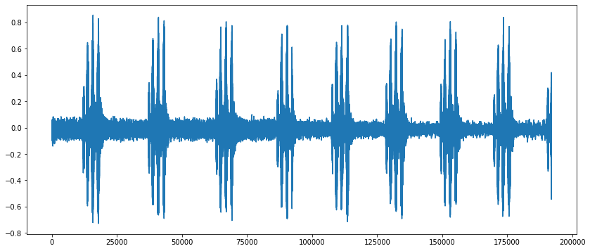
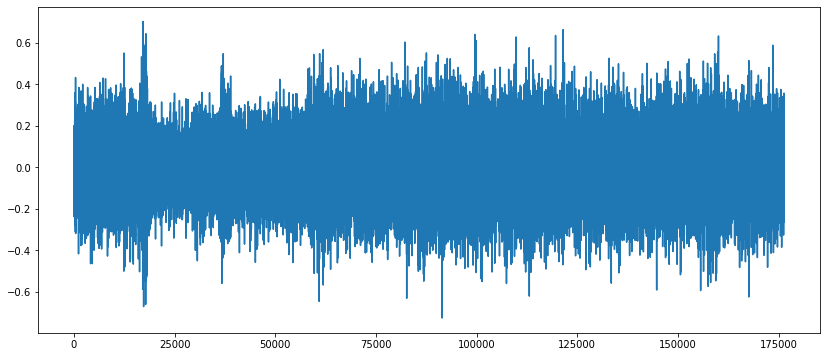
The data used for this demonstration comes from the Urban Sounds Dataset. This dataset and its taxonomy is presented in J. Salamon, C. Jacoby and J. P. Bello, A Dataset and Taxonomy for Urban Sound Research, 22nd ACM International Conference on Multimedia, Orlando USA, Nov. 2014.

For simplicity the dataset is sampled and a subset of 20 audio clips from two categories are used - air conditioner (AC) and drill.

1
ZipFile.namelist(zip_file)
['audio_data/',
 'audio_data/ac/',
 'audio_data/ac/101729-0-0-1.wav',
 'audio_data/ac/101729-0-0-11.wav',
 'audio_data/ac/101729-0-0-12.wav',
 'audio_data/ac/101729-0-0-13.wav',
 'audio_data/ac/101729-0-0-14.wav',
 'audio_data/ac/101729-0-0-16.wav',
 'audio_data/ac/101729-0-0-17.wav',
 'audio_data/ac/101729-0-0-18.wav',
 'audio_data/ac/101729-0-0-19.wav',
 'audio_data/ac/101729-0-0-21.wav',
 'audio_data/ac/101729-0-0-22.wav',
 'audio_data/ac/101729-0-0-23.wav',
 'audio_data/ac/101729-0-0-24.wav',
 'audio_data/ac/101729-0-0-26.wav',
 'audio_data/ac/101729-0-0-28.wav',
 'audio_data/ac/101729-0-0-29.wav',
 'audio_data/ac/101729-0-0-3.wav',
 'audio_data/ac/101729-0-0-32.wav',
 'audio_data/ac/101729-0-0-33.wav',
 'audio_data/ac/101729-0-0-36.wav',
 'audio_data/drill/',
 'audio_data/drill/103199-4-0-0.wav',
 'audio_data/drill/103199-4-0-3.wav',
 'audio_data/drill/103199-4-0-4.wav',
 'audio_data/drill/103199-4-0-5.wav',
 'audio_data/drill/103199-4-0-6.wav',
 'audio_data/drill/103199-4-1-0.wav',
 'audio_data/drill/103199-4-2-0.wav',
 'audio_data/drill/103199-4-2-1.wav',
 'audio_data/drill/103199-4-2-10.wav',
 'audio_data/drill/103199-4-2-11.wav',
 'audio_data/drill/103199-4-2-2.wav',
 'audio_data/drill/103199-4-2-3.wav',
 'audio_data/drill/103199-4-2-4.wav',
 'audio_data/drill/103199-4-2-5.wav',
 'audio_data/drill/103199-4-2-6.wav',
 'audio_data/drill/103199-4-2-7.wav',
 'audio_data/drill/103199-4-2-8.wav',
 'audio_data/drill/103199-4-2-9.wav',
 'audio_data/drill/103199-4-4-0.wav',
 'audio_data/drill/103199-4-6-0.wav']
1
2
3
4
5
6
7
8
9
10
11
12
13
14
15
16
17
18
19
20
21
22
23
24
25
26
audio_data = []
labels = []
sampling_rate = []
file_names = []

for file_name in ZipFile.namelist(zip_file):
# Skip directories
if not os.path.basename(file_name):
continue

audio_file = None
if file_name.startswith("audio_data/ac/"):
labels.append(0)
audio_file = zip_file.open(file_name)
elif file_name.startswith("audio_data/drill/"):
labels.append(1)
audio_file = zip_file.open(file_name)
else:
print("Unknown file class. Skipping.")

if audio_file is not None:
file_names.append(file_name)
tmp = BytesIO(audio_file.read())
data, samplerate = sf.read(tmp)
audio_data.append(data)
sampling_rate.append(samplerate)
1
len(audio_data),audio_data[0].shape
(40, (192000, 2))
1
2
3
from collections import Counter

Counter(labels)
Counter({0: 20, 1: 20})
1
2
3
4
5
# for index in range(len(audio_data)):

# if (sampling_rate[index] == 48000):
# audio_data[index] = librosa.resample(audio_data[index], 48000, 44100)
# sampling_rate[index] = 44100
1
2
3
4
5
6
7
def to_mono(data):
if data.ndim > 1:
data = np.mean(data, axis=1)
return data

for index in range(len(audio_data)):
audio_data[index] = to_mono(audio_data[index])
1
2
fig = plt.figure(figsize=(14,6))
plt.plot(audio_data[0])
[<matplotlib.lines.Line2D at 0x159e6f6d8>]
png
1
2
fig = plt.figure(figsize=(14,6))
plt.plot(audio_data[21])
[<matplotlib.lines.Line2D at 0x12fce4be0>]
png
1
2
3
scales = np.arange(1, 101)
coeff1, freqs1 = pywt.cwt(audio_data[1][:25000], scales, 'morl')
coeff2, freqs2 = pywt.cwt(audio_data[21][:25000], scales, 'morl')
1
coeff1.shape, freqs1.shape
((100, 25000), (100,))
1
2
3
4
5
6
7
plt.figure(1, figsize=(20,10))
plt.subplot(121)
plt.imshow(coeff1, cmap='coolwarm', aspect='auto')
plt.subplot(122)
plt.imshow(coeff2, cmap='coolwarm', aspect='auto')

plt.show()
png
1
2
3
4
5
6
7
8
9
10
11
12
13
14
15
16
17
18
19
20
21
22
23
24
25
26
27
28
29
30
31
import matplotlib.pyplot as plt
from mpl_toolkits.mplot3d import Axes3D
from matplotlib import cm

fig = plt.figure(figsize=(40,15))

ax1 = fig.add_subplot(1, 2, 1, projection='3d')

Y = np.arange(1, 101, 1)
X = np.arange(1, 25001, 1)

X, Y = np.meshgrid(X, Y)

ax1.plot_surface(X, Y, coeff1, cmap=cm.coolwarm, linewidth=0, antialiased=True)

ax1.set_xlabel("Time", fontsize=20)
ax1.set_ylabel("Scale", fontsize=20)
ax1.set_zlabel("Amplitude", fontsize=20)
ax1.set_zlim3d(-1,1)

ax2 = fig.add_subplot(1, 2, 2, projection='3d')

ax2.plot_surface(X, Y, coeff2, cmap=cm.coolwarm, linewidth=0, antialiased=True)


ax2.set_xlabel("Time", fontsize=20)
ax2.set_ylabel("Scale", fontsize=20)
ax2.set_zlabel("Amplitude", fontsize=20)
ax2.set_zlim3d(-1,1)

plt.show()
png
1
2
3
4
5
6
7
8
9
10
11
from sklearn.decomposition import PCA

pca = PCA(n_components=1)

features = np.empty((0,100))

for ind in range(len(audio_data)):
print('.', end='')
coeff, freqs = pywt.cwt(audio_data[ind][:25000], scales, 'morl')
features = np.vstack([features, pca.fit_transform(coeff).flatten()])

........................................
1
X_train, X_test, y_train, y_test = train_test_split(features, labels, test_size=0.20, random_state=0)
1
2
clf = svm.SVC()
clf.fit(X_train, y_train)
SVC(C=1.0, break_ties=False, cache_size=200, class_weight=None, coef0=0.0,
    decision_function_shape='ovr', degree=3, gamma='scale', kernel='rbf',
    max_iter=-1, probability=False, random_state=None, shrinking=True,
    tol=0.001, verbose=False)
1
2
y_pred = clf.predict(X_test)
print("Accuracy : %.2f%%" % (accuracy_score(y_test, y_pred) * 100))
Accuracy : 87.50%