1 | import numpy as np |
Uniform distribution(continuous)
- Uniform distribution has same probaility value on [a, b], easy probability.
\[f(x)=\begin{cases} \frac{1}{b - a} & \mathrm{for}\ a \le x \le b, \\[8pt] 0 & \mathrm{for}\ x<a\ \mathrm{or}\ x>b \end{cases}\]
1 | def uniform(x, a, b): |
1 | s = np.random.uniform(0,1,1000) |
[<matplotlib.lines.Line2D at 0x11eae0cc0>]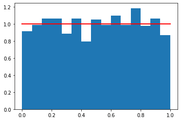
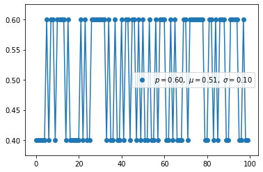
Bernoulli distribution(discrete)
- Bernoulli distribution is not considered about prior probability P(X). Therefore, if we optimize to the maximum likelihood, we will be vulnerable to overfitting.
- We use binary cross entropy to classify binary classification. It has same form like taking a negative log of the bernoulli distribution.
\[f(k;p) = \begin{cases} p & \text{if }k=1, \\ q = 1-p & \text {if } k = 0. \end{cases}\]
- For Logistic Regression \[p=p(y|x,\theta)=p_{1}^{y_{i}}\ast p_{0}^{1-y_{i}}\] \[max \sum_{i=1}^{m}({y_{i}\log{p_{1}}+(1-y_{i})\log{p_{0})}}\]
1 | def bernoulli(p, k): |
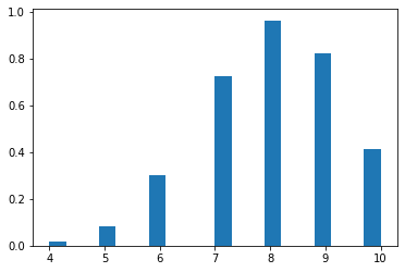
Binomial distribution(discrete)
- Binomial distribution with parameters n and p is the discrete probability distribution of the number of successes in a sequence of n independent experiments.
- Binomial distribution is distribution considered prior probaility by specifying the number to be picked in advance.
\[f(k,n,p) = \Pr(k;n,p) = \Pr(X = k) = \binom{n}{k}p^k(1-p)^{n-k}\]
for k = 0, 1, 2, ..., n, where \[\binom{n}{k} =\frac{n!}{k!(n-k)!}\]
1 | def const(n, r): |
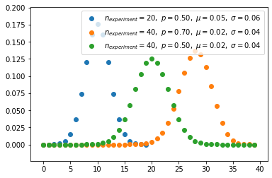
1 | s = np.random.binomial(10, 0.8, 1000) |
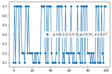
Multi-Bernoulli distribution, Categorical distribution(discrete)
- Multi-bernoulli called categorical distribution, is a probability expanded more than 2.
- cross entopy has same form like taking a negative log of the Multi-Bernoulli distribution.
\[f(x\mid \boldsymbol{p} ) = \prod_{i=1}^k p_i^{[x=i]}\] where \([x = i]\) evaluates to 1 if \(x = i\), 0 otherwise. There are various advantages of this formulation
1 | def categorical(p, k): |
Multinomial distribution(discrete)
- The multinomial distribution has the same relationship with the categorical distribution as the relationship between Bernoull and Binomial.
- For example, it models the probability of counts for each side of a k-sided die rolled n times. For n independent trials each of which leads to a success for exactly one of k categories, with each category having a given fixed success probability, the multinomial distribution gives the probability of any particular combination of numbers of successes for the various categories.
- When k is 2 and n is 1, the multinomial distribution is the Bernoulli distribution. When k is 2 and n is bigger than 1, it is the binomial distribution. When k is bigger than 2 and n is 1, it is the categorical distribution.
\[\begin{align} f(x_1,\ldots,x_k;n,p_1,\ldots,p_k) & {} = \Pr(X_1 = x_1 \text{ and } \dots \text{ and } X_k = x_k) \\ & {} = \begin{cases} { \displaystyle {n! \over x_1!\cdots x_k!}p_1^{x_1}\times\cdots\times p_k^{x_k}}, \quad & \text{when } \sum_{i=1}^k x_i=n \\ \\ 0 & \text{otherwise,} \end{cases} \end{align}\] for non-negative integers \(x_1, \cdots, x_k\).
The probability mass function can be expressed using the gamma function as:
\[f(x_1,\dots, x_{k}; p_1,\ldots, p_k) = \frac{\Gamma(\sum_i x_i + 1)}{\prod_i \Gamma(x_i+1)} \prod_{i=1}^k p_i^{x_i}.\]
1 | def factorial(n): |
1 | np.random.multinomial(20, [1/6.]*6, size=10) |
array([[1, 1, 2, 3, 8, 5],
       [2, 4, 3, 3, 6, 2],
       [1, 6, 3, 2, 3, 5],
       [5, 3, 4, 4, 2, 2],
       [3, 8, 4, 2, 0, 3],
       [2, 4, 1, 5, 1, 7],
       [6, 3, 2, 4, 3, 2],
       [8, 2, 1, 1, 4, 4],
       [3, 6, 4, 1, 4, 2],
       [3, 2, 3, 3, 6, 3]])
Beta distribution(continuous)
- Beta distribution is conjugate to the binomial and Bernoulli distributions.
- Using conjucation, we can get the posterior distribution more easily using the prior distribution we know.
- Uniform distiribution is same when beta distribution met special case(alpha=1, beta=1).
\[\begin{align} f(x;\alpha,\beta) & = \mathrm{constant}\cdot x^{\alpha-1}(1-x)^{\beta-1} \\[3pt] & = \frac{x^{\alpha-1}(1-x)^{\beta-1}}{\displaystyle \int_0^1 u^{\alpha-1} (1-u)^{\beta-1}\, du} \\[6pt] & = \frac{\Gamma(\alpha+\beta)}{\Gamma(\alpha)\Gamma(\beta)}\, x^{\alpha-1}(1-x)^{\beta-1} \\[6pt] & = \frac{1}{B(\alpha,\beta)} x^{\alpha-1}(1-x)^{\beta-1} \end{align}\]
1 | def gamma_function(n): |
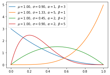
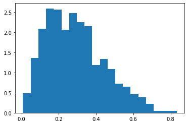
1 | s = np.random.beta(2, 5, size=1000) |
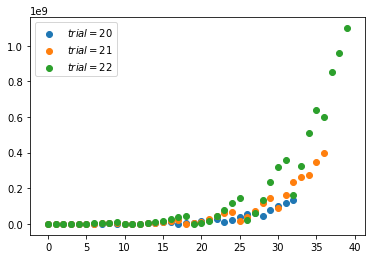
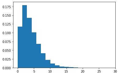
Gamma distribution(continuous)
Gamma distribution will be beta distribution, if \(\frac{Gamma(a,1)}{Gamma(a,1) + Gamma(b,1)}\) is same with \(Beta(a,b)\).
The exponential distribution and chi-squared distribution are special cases of the gamma distribution.
A random variable X that is gamma-distributed with shape α and rate β is denoted: \[X \sim \Gamma(\alpha, \beta) \equiv \operatorname{Gamma}(\alpha,\beta)\] The corresponding probability density function in the shape-rate parametrization is: \[\begin{align} f(x;\alpha,\beta) & = \frac{ \beta^\alpha x^{\alpha-1} e^{-\beta x}}{\Gamma(\alpha)} \quad \text{ for } x > 0 \quad \alpha, \beta > 0, \\[6pt] \end{align}\]
1 | def gamma_function(n): |
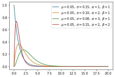
1 | a, b = 2., 2. |
[<matplotlib.lines.Line2D at 0x12cb80c50>]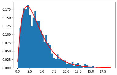
Dirichlet distribution(continuous)
- Dirichlet distribution is conjugate to the MultiNomial distributions. 即Dirichlet分布乘上一个多项分布的似然函数后,得到的后验分布仍然是一个Dirichlet分布。
- If k=2, it will be Beta distribution.
\[f \left(x_1,\ldots, x_{K}; \alpha_1,\ldots, \alpha_K \right) = \frac{1}{\mathrm{B}(\boldsymbol\alpha)} \prod_{i=1}^K x_i^{\alpha_i - 1}\]
where \(\{x_k\}\_{k=1}^{k=K}\) belong to the standard \(K-1\) simplex, or in other words:
\[\sum_{i=1}^{K} x_i=1 \mbox{ and } x_i \ge 0 \mbox{ for all } i \in [1,K]\]
The normalizing constant is the multivariate beta function, which can be expressed in terms of the gamma function
\[\mathrm{B}(\boldsymbol\alpha) = \frac{\prod_{i=1}^K \Gamma(\alpha_i)}{\Gamma\left(\sum_{i=1}^K \alpha_i\right)},\qquad\boldsymbol{\alpha}=(\alpha_1,\ldots,\alpha_K).\]
Dirichlet分布可以看做是分布之上的分布。如何理解这句话,我们可以先举个例子:假设我们有一个骰子,其有六面,分别为{1,2,3,4,5,6}。现在我们做了10000次投掷的实验,得到的实验结果是六面分别出现了{2000,2000,2000,2000,1000,1000}次,如果用每一面出现的次数与试验总数的比值估计这个面出现的概率,则我们得到六面出现的概率,分别为{0.2,0.2,0.2,0.2,0.1,0.1}。现在,我们还不满足,我们想要做10000次试验,每次试验中我们都投掷骰子10000次。我们想知道,骰子六面出现概率为{0.2,0.2,0.2,0.2,0.1,0.1}的概率是多少(说不定下次试验统计得到的概率为{0.1, 0.1, 0.2, 0.2, 0.2, 0.2}这样了)。这样我们就在思考骰子六面出现概率分布这样的分布之上的分布。而这样一个分布就是Dirichlet分布。
1 | def normalization(x, s): |
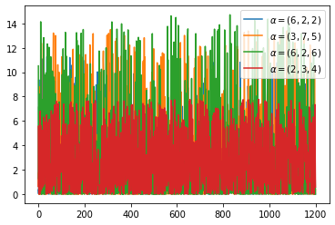
1 | s = np.random.dirichlet((0.2, 0.3, 0.5), 20).transpose() |
1 | s.shape |
(3, 20)1 | plt.barh(range(20), s[0]) |
<BarContainer object of 20 artists>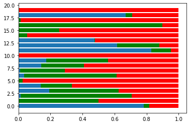
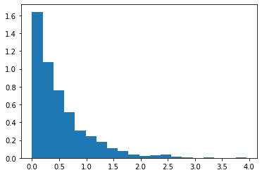
Exponential distribution(continuous)
- Exponential distribution is special cases of the gamma distribution when alpha is 1.
\[f(x;\lambda) = \begin{cases} \lambda e^{-\lambda x} & x \ge 0, \\ 0 & x < 0. \end{cases}\]
1 | def exponential(x, lamb): |
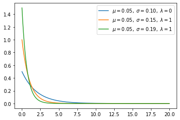
1 | s = np.random.exponential(scale = 0.5, size=1000) |
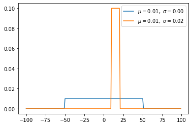
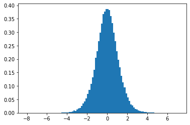
Gaussian distribution(continuous)
\[f(x) = \frac{1}{\sigma \sqrt{2\pi} } e^{-\frac{1}{2}\left(\frac{x-\mu}{\sigma}\right)^2}\]
1 | def gaussian(x, n): |
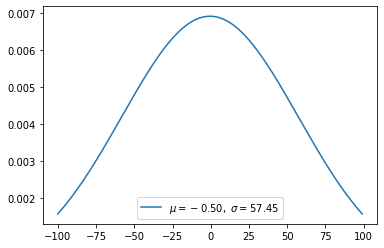
1 | mu, sigma = 0, 0.1 # mean and standard deviation |
[<matplotlib.lines.Line2D at 0x11122d4e0>]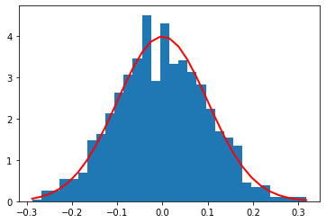
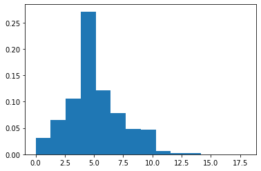
Poisson distribution
- 在一个时间段内事件平均发生的次数服从泊松分布
\[\!f(k; \lambda)= \Pr(X = k)= \frac{\lambda^k e^{-\lambda}}{k!},\] - e is Euler's number (e = 2.71828...) - k! is the factorial of k.
1 | s = np.random.poisson(5, 10000) |
Chi-squared distribution(continuous)
- Chi-square distribution with k degrees of freedom is the distribution of a sum of the squares of k independent standard normal random variables.
- Chi-square distribution is special case of Beta distribution
If \(Z_1, \cdots, Z_k\) are independent, standard normal random variables, then the sum of their squares,
\[Q\ = \sum_{i=1}^k Z_i^2 ,\]
is distributed according to the chi-square distribution with k degrees of freedom. This is usually denoted as
\[Q\ \sim\ \chi^2(k)\ \ \text{or}\ \ Q\ \sim\ \chi^2_k .\]
The chi-square distribution has one parameter: a positive integer k that specifies the number of degrees of freedom (the number of \(Z_i\) s).
The probability density function (pdf) of the chi-square distribution is
\[f(x;\,k) = \begin{cases} \dfrac{x^{\frac k 2 -1} e^{-\frac x 2}}{2^{\frac k 2} \Gamma\left(\frac k 2 \right)}, & x > 0; \\ 0, & \text{otherwise}. \end{cases}\]
1 | def gamma_function(n): |
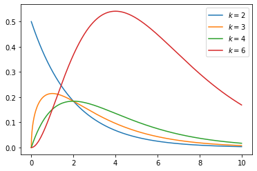
1 | s = np.random.chisquare(4,10000) |
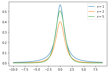
Student-t distribution(continuous)
- Definition
Let \(X_1, \cdots, X_n\) be independent and identically distributed as \(N(\mu, \sigma^2)\), i.e. this is a sample of size \(n\) from a normally distributed population with expected mean value \(\mu\) and variance \(\sigma^{2}\)
Let \[\bar X = \frac 1 n \sum_{i=1}^n X_i\] be the sample mean and let \[S^2 = \frac 1 {n-1} \sum_{i=1}^n (X_i - \bar X)^2\]
be the (Bessel-corrected) sample variance.
Then the random variable \[\frac{ \bar X - \mu} {S /\sqrt{n}}\]
has a standard normal distribution
Student's t-distribution has the probability density function given by
\[f(t) = \frac{\Gamma(\frac{\nu+1}{2})} {\sqrt{\nu\pi}\,\Gamma(\frac{\nu}{2})} \left(1+\frac{t^2}{\nu} \right)^{\!-\frac{\nu+1}{2}}\]
- \(\nu\) is the number of degrees of freedom
- \(\Gamma\) is the gamma function.
1 | def gamma_function(n): |
1 | ## Suppose the daily energy intake for 11 women in kilojoules (kJ) is: |
So the p-value is about 0.009, which says the null hypothesis has a probability of about 99% of being true.
1 | np.sum(s<t) / float(len(s)) |
0.0086Reference
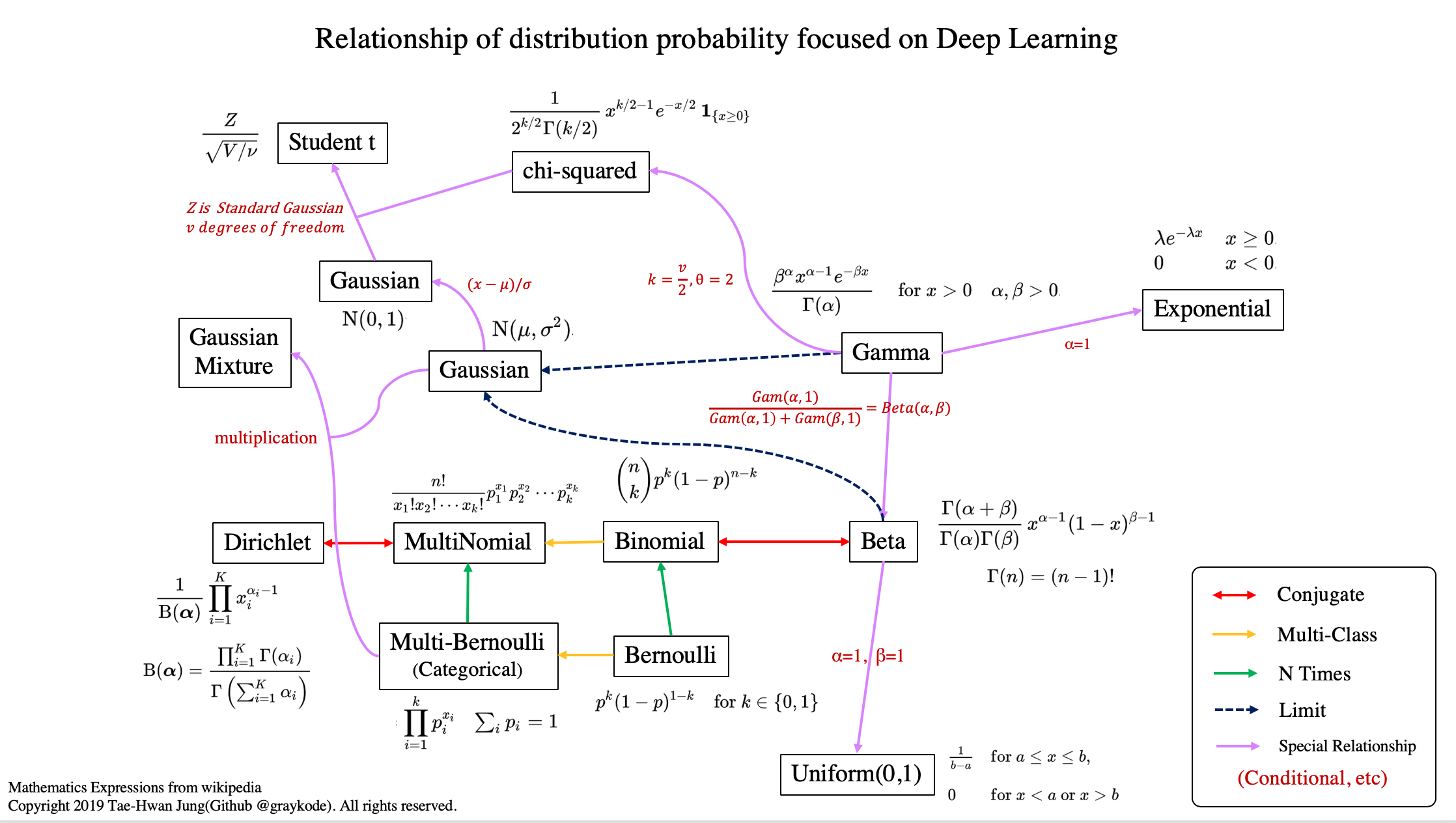
- https://github.com/graykode/distribution-is-all-you-need
- https://blog.csdn.net/deropty/article/details/50266309