reference from Matrix Algebra for Engineers by Jeffrey R. Chasnov
Vector spaces
- A vector space consists of a set of vectors and a set of scalars.
- For the set of vectors and scalars to form a vector space, the set of vectors must be closed under vector addition and scalar multiplication. That is, when you multiply any two vectors in the set by real numbers and add them, the resulting vector must still be in the set.
As an example: \[ \begin{pmatrix} \mu_{1} \\ \mu_{2} \\ \mu_{3} \\ \end{pmatrix}, \begin{pmatrix} \nu_{1} \\ \nu_{2} \\ \nu_{3} \\ \end{pmatrix} \]
then
\[ w = a\mu + b\nu = \begin{pmatrix} a\mu_{1} + b\nu_{1} \\ a\mu_{2} + b\nu_{2} \\ a\mu_{3} + b\nu_{3} \\ \end{pmatrix} \]
so that the set of all three-by-one matrices (together with the set of real numbers) is a vector space. This space is usually called .
Linear independence
The set of vectors, \({u_{1}, u_{2}, . . . , u_{n}}\), are linearly independent if for any scalars \(c_{1}, c_{2}, . . . , c_{n}\), the equation
\[c_{1}u_{1}+c_{2}u_{2}+···+c_{n}u_{n} = 0\]
has only the solution \(c_{1} = c_{2} = ··· = c_{n} = 0\)
Span, basis and dimension
Span
Given a set of vectors, one can generate a vector space by forming all linear combinations of that set of vectors. The span of the set of vectors \({v_{1}, v_{2}, . . . , v_{n}}\) is the vector space consisting of all linear combinations of \(v_{1}, v_{2}, . . . , v_{n}\). We say that a set of vectors spans a vector space.
basis
The smallest set of vectors needed to span a vector space forms a basis for that vector space
dimension
The number of vectors in a basis gives the dimension of the vector space
Gram-Schmidt process
Given any basis for a vector space, we can use an algorithm called the Gram-Schmidt process to construct an orthonormal basis for that space
Let the vectors \(v_{1}, v_{2}, . . . , v_{n}\) be a basis for some n- dimensional vector space. We will assume here that these vectors are column matrices, but this process also applies more generally. We will construct an orthogonal basis \(u_{1}, u_{2}, . . . , u_{n}\), and then normalize each vector to obtain an orthonormal basis.
First, define \(u_{1} = v_{1}\), To find the next orthogonal basis vector, define
\[ u_{2} = v_{2} - \frac{(u_{1}^{T}v_{2})u_{1}}{u_{1}^{T}u_{1}} \]
The next orthogonal vector in the new basis can be found from \[ u_{3} = v_{3} - \frac{(u_{1}^{T}v_{3})u_{1}}{u_{1}^{T}u_{1}} - \frac{(u_{2}^{T}v_{3})u_{2}}{u_{2}^{T}u_{2}} \]
We can continue in this fashion to construct n orthogonal basis vectors. These vectors can then be normalized via \[ \hat{u_{1}} = \frac{u_{1}}{(u_{1}^{T}u_{1})^{\frac{1}{2}}} \]
Null space
The null space of a matrix A, which we denote as Null(A), is the vector space spanned by all column vectors x that satisfy the matrix equation
\[Ax = 0\]
To find a basis for the null space of a noninvertible matrix, we bring A to reduced row echelon form. \[ A = \begin{pmatrix} -3 & 6 & -1 & 1 & -1 \\ 1 & -2 & 2 & 3 & -1 \\ 2 & -4 & 5 & 8 & -4 \\ \end{pmatrix} \rightarrow A = \begin{pmatrix} 1 & -2 & 0 & -1 & 3 \\ 0 & 0 & 1 & 2 & -2 \\ 0 & 0 & 0 & 0 & 0 \\ \end{pmatrix} \]
We call the variables associated with the pivot columns, x1 and x3, basic variables, and the variables associated with the non-pivot columns, x2, x4 and x5, free variables. Writing the basic variables on the left-hand side of the \(Ax = 0\) equations, we have from the first and second rows
\[ \begin{align*} x_{1} = 2x_{2} + x_{4} - 3x_{5}, \\ x_{3} = -2x_{4} + 2x_{5}, \\ \end{align*} \]
Eliminating x1 and x3, we can write the general solution for vectors in Null(A) as
\[ \begin{pmatrix} 2x_{2} + x_{4} - 3x_{5} \\ x_{2} \\ -2x_{4} + 2x_{5} \\ x_{4} \\ x_{5} \\ \end{pmatrix} = x_{2} \begin{pmatrix} 2 \\ 1 \\ 0 \\ 0 \\ 0 \\ \end{pmatrix} + x_{4} \begin{pmatrix} 1 \\ 0 \\ -2 \\ 1 \\ 0 \\ \end{pmatrix} + x_{5} \begin{pmatrix} -3 \\ 0 \\ 2 \\ 0 \\ 1 \\ \end{pmatrix} \]
where the free variables \(x_{2}\), \(x_{4}\), and \(x_{5}\) can take any values. By writing the null space in this form, a basis for Null(A) is made evident, and is given by
\[ \left\{ \begin{pmatrix} 2 \\ 1 \\ 0 \\ 0 \\ 0 \\ \end{pmatrix}, \begin{pmatrix} 1 \\ 0 \\ -2 \\ 1 \\ 0 \\ \end{pmatrix}, \begin{pmatrix} -3 \\ 0 \\ 2 \\ 0 \\ 1 \\ \end{pmatrix} \right\} \]
Application of the null space
An underdetermined system of linear equations \(Ax = b\) with more unknowns than equations may not have a unique solution
If u is the general form of a vector in the null space of A, and v is any vector that satisfies \(Av = b\), then \(x = u+v\) satisfies \(Ax = A(u+v) = Au+Av = 0+b = b\). The general solution of \(Ax = b\) can therefore be written as the sum of a general vector in Null(A) and a particular vector that satisfies the underdetermined system.
As an example,
\[ \begin{align*} 2x_{1} + 2x_{2} + x_{3} = 0, \\ 2x_{1} − 2x_{2} − x_{3} = 1, \\ \end{align*} \]
We first bring the augmented matrix to reduced row echelon form:
\[ \begin{pmatrix} 2 & 2 & 1 & 0 \\ 2 & -2 & -1 & 1 \\ \end{pmatrix} \rightarrow \begin{pmatrix} 1 & 0 & 0 & \frac{1}{4} \\ 0 & 1 & \frac{1}{2} & -\frac{1}{4} \\ \end{pmatrix} \]
The null space is determined from \(x_{1} = 0\) and \(x_{2} = −\frac{x_{3}}{2}\), and we can write
\[ Null(A) = span \left\{ \begin{pmatrix} 0 \\ -1 \\ 2 \end{pmatrix}\right\} \]
The general solution to the original underdetermined linear system is the sum of the null space and the particular solution and is given by
\[ \begin{pmatrix} x_{1} \\ x_{2} \\ x_{3} \\ \end{pmatrix} = a \begin{pmatrix} 0 \\ -1 \\ 2 \\ \end{pmatrix} + \frac{1}{4} \begin{pmatrix} 1 \\ -1 \\ 0 \\ \end{pmatrix} \]
Column space
The column space of a matrix is the vector space spanned by the columns of the matrix. When a matrix is multiplied by a column vector, the resulting vector is in the column space of the matrix, as can be seen from
\[ \begin{pmatrix} a & b \\ c & d \\ \end{pmatrix} \begin{pmatrix} x \\ y \\ \end{pmatrix} = \begin{pmatrix} ax + by \\ cx + dy \\ \end{pmatrix} = x \begin{pmatrix} a \\ c \\ \end{pmatrix} + y \begin{pmatrix} b \\ d \\ \end{pmatrix} \]
Recall that the dimension of the null space is the number of non-pivot columns—equal to the number of free variables—so that the sum of the dimensions of the null space and the column space is equal to the total number of columns—equal
\[dim(Col(A)) + dim(Null(A)) = n.\]
Row space, left null space and rank
In addition to the column space and the null space, a matrix A has two more vector spaces associated with it, namely the column space and null space of \(A^{T}\), which are called the row space and the left null space.
Furthermore, the dimension of the column space of A is also equal to the number of pivot columns, so that the dimensions of the column space and the row space of a matrix are equal. We have \[dim(Col(A)) = dim(Row(A)).\]
We call this dimension the rank of the matrix A
Orthogonal projections
Suppose that V is an n-dimensional vector space and W is a p-dimensional subspace of V. In general, the orthogonal projection of v onto W is given by \[ v_{proj_{W}} = (v^{T}s_{1})s_{1} + (v^{T}s_{2})s_{2} + · · · + (v^{T}s_{p})s_{p}; \]
and we can write \[v=v_{proj_{W}} +(v−v_{proj_{W}})\]
\(v_{proj_{W}}\) is closer to v than any other vector in W
The least-squares problem
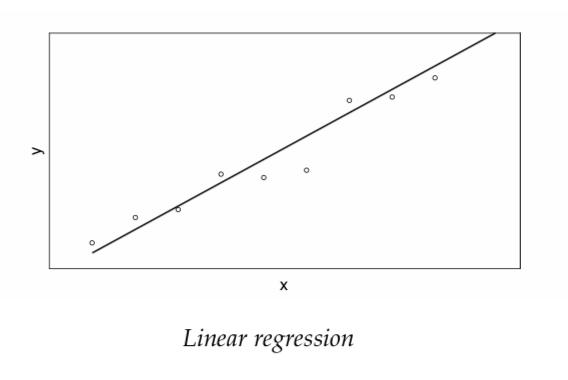
These equations constitute a system of n equations in the two unknowns \(\beta_{0}\) and \(\beta_{1}\). The corresponding matrix equation is given by: \[ \begin{pmatrix} 1 & x_{1} \\ 1 & x_{2} \\ \vdots \\ 1 & x_{n} \\ \end{pmatrix} \begin{pmatrix} \beta{0} \\ \beta{1} \\ \end{pmatrix} = \begin{pmatrix} y_{1} \\ y_{2} \\ \vdots \\ y_{n} \end{pmatrix} \]
This is an overdetermined system of equations with no solution. The problem of least squares is to find the best solution.
We can generalize this problem as follows. Suppose we are given a matrix equation, \(Ax = b\), that has no solution because b is not in the column space of A. So instead we solve \(Ax = b_{projCol(A)}\) , where \(b_{projCol(A)}\) is the projection of b onto the column space of A. The solution is then called the least-squares solution for x.
\[b_{projCol(A)} = A(A^{T}A)^{−1}A^{T}b.\]
Laplace expansion
\[ \begin{vmatrix} a & b & c \\ d & e & f \\ g & h & i \\ \end{vmatrix} = aei+bfg+cdh−ceg−bdi−afh = a(ei− fh)−b(di− fg)+c(dh−eg) \\ \]
which can be written suggestively as
\[ \begin{vmatrix} a & b & c \\ d & e & f \\ g & h & i \\ \end{vmatrix} = a \begin{vmatrix} e & f \\ h & i \\ \end{vmatrix} - b \begin{vmatrix} d & f \\ g & i \\ \end{vmatrix} + c \begin{vmatrix} d & e \\ g & h \\ \end{vmatrix} \]
Properties of a determinant
- Property 1: The determinant of the identity matrix is one;
- Property 2: The determinant changes sign under row interchange;
- Property 3: The determinant is a linear function of the first row, holding all other rows fixed.
The eigenvalue problem
Let A be a square matrix, x a column vector, and λ a scalar. The eigenvalue problem for A solves
\[Ax = \lambda x\]
for eigenvalues \(\lambda_{i}\) with corresponding eigenvectors \(x_{i}\). Making use of the identity matrix I, the eigenvalue problem can be rewritten as
\[(A−\lambda I)x = 0\]
For there to be nonzero eigenvectors, the matrix \((A − \lambda I)\) must be singular, that is,
\[det(A−\lambda I) = 0.\]
Matrix diagonalization
For concreteness, consider a two-by-two matrix A with eigenvalues and eigenvectors given by
\[ \lambda_{1}, x_{1} = \begin{pmatrix} x_{11}\\ x_{21}\\ \end{pmatrix} ; \lambda_{2}, x_{2} = \begin{pmatrix} x_{12}\\ x_{22}\\ \end{pmatrix} \]
And consider the matrix product and factorization given by
\[ A \begin{pmatrix} x_{11} & x_{12} \\ x_{21} & x_{22} \\ \end{pmatrix} = \begin{pmatrix} \lambda_{1}x_{11} & \lambda_{2}x_{12} \\ \lambda_{1}x_{21} & \lambda_{2}x_{22} \\ \end{pmatrix} = \begin{pmatrix} x_{11} & x_{12} \\ x_{21} & x_{22} \\ \end{pmatrix} \begin{pmatrix} \lambda_{1} & 0 \\ 0 & \lambda_{2} \\ \end{pmatrix} \]
Generalizing, we define S to be the matrix whose columns are the eigenvectors of A, and Λ to be the diagonal matrix with eigenvalues down the diagonal. Then for any n-by-n matrix with n linearly independent eigenvectors, we have
\[AS = SΛ\]
where S is an invertible matrix. Multiplying both sides on the right or the left by \(S^{−1}\), we derive the relations
\[A = SΛS^{−1} \quad or \quad Λ = S^{−1}AS.\]
Powers of a matrix
Suppose that A is diagonalizable, and consider \[A^{p} = (SΛS^{−1})(SΛS^{−1}) = SΛ^{p}S^{−1}\]
\[ \begin{pmatrix} \lambda_{1} & 0 \\ 0 & \lambda_{2} \\ \end{pmatrix} \begin{pmatrix} \lambda_{1} & 0 \\ 0 & \lambda_{2} \\ \end{pmatrix} = \begin{pmatrix} \lambda_{1}^{2} & 0 \\ 0 & \lambda_{2}^{2} \\ \end{pmatrix} \]