Applications
Route finding
- Route finding is perhaps the most canonical example of a search problem. We are given as the input a map, a source point and a destination point. The goal is to output a sequence of actions (e.g., go straight, turn left, or turn right) that will take us from the source to the destination.
- We might evaluate action sequences based on an objective (distance, time, or pleasantness).
Robot motion planning
- In robot motion planning, the goal is get a robot to move from one position/pose to another. The desired output trajectory consists of individual actions, each action corresponding to moving or rotating the joints by a small amount.
- Again, we might evaluate action sequences based on various resources like time or energy.
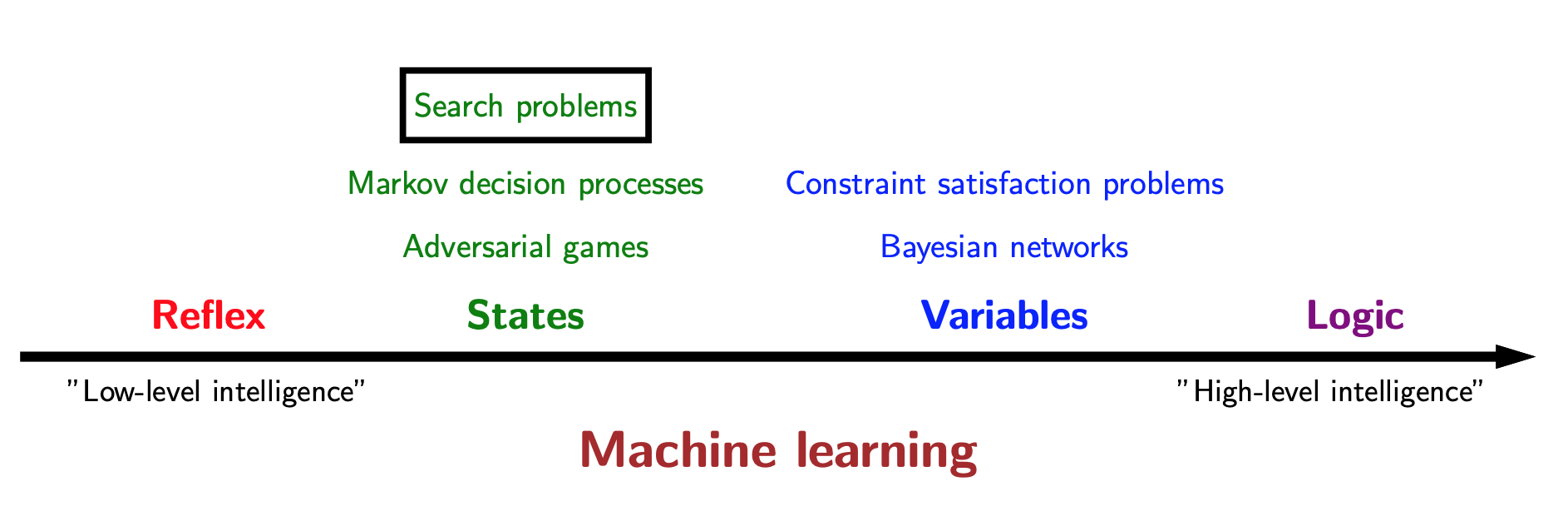
Search Problems
- Recall the modeling-inference-learning paradigm. For reflex-based classifiers, modeling consisted of choos- ing the features and the neural network architecture; inference was trivial forward computation of the output given the input; and learning involved using stochastic gradient descent on the gradient of the loss function, which might involve backpropagation.
- Today, we will focus on the modeling and inference part of search problems. The next lecture will cover learning.
Definitions
- \(S_{start}\): staring state$
- Actions(s): possible actions
- Cons(s,a): action cost
- Succ(s,a): successor
- IsEnd(s): reached end state?
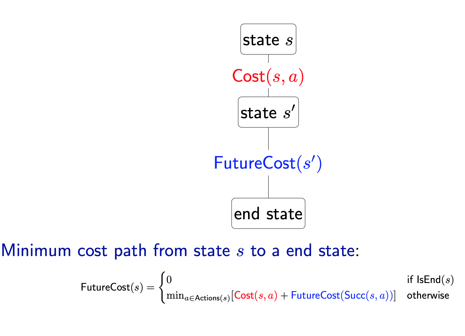
We will build what we will call a search tree. The root of the tree is the start state $S_{start}$, and the leaves are the end states (IsEnd(s) is true). Each edge leaving a node s corresponds to a possible action $a \in \text{Actions(s)}$ that could be performed in state s. The edge is labeled with the action and its cost, written a : Cost(s,a). The action leads deterministically to the successor state Succ(s,a), represented by the child node.
In summary, each root-to-leaf path represents a possible action sequence, and the sum of the costs of the edges is the cost of that path. The goal is to find the root-to-leaf path that ends in a valid end state with minimum cost.
Note that in code, we usually do not build the search tree as a concrete data structure. The search tree is used merely to visualize the computation of the search algorithms and study the structure of the search problem.
Transportation example
1 | Street with blocks numbered 1 to n. |
1 | class TransportationProblem(object): |
Now let’s put modeling aside and suppose we are handed a search problem. How do we construct an algorithm for finding a minimum cost path (not necessarily unique)?
Tree search
Backtracking search
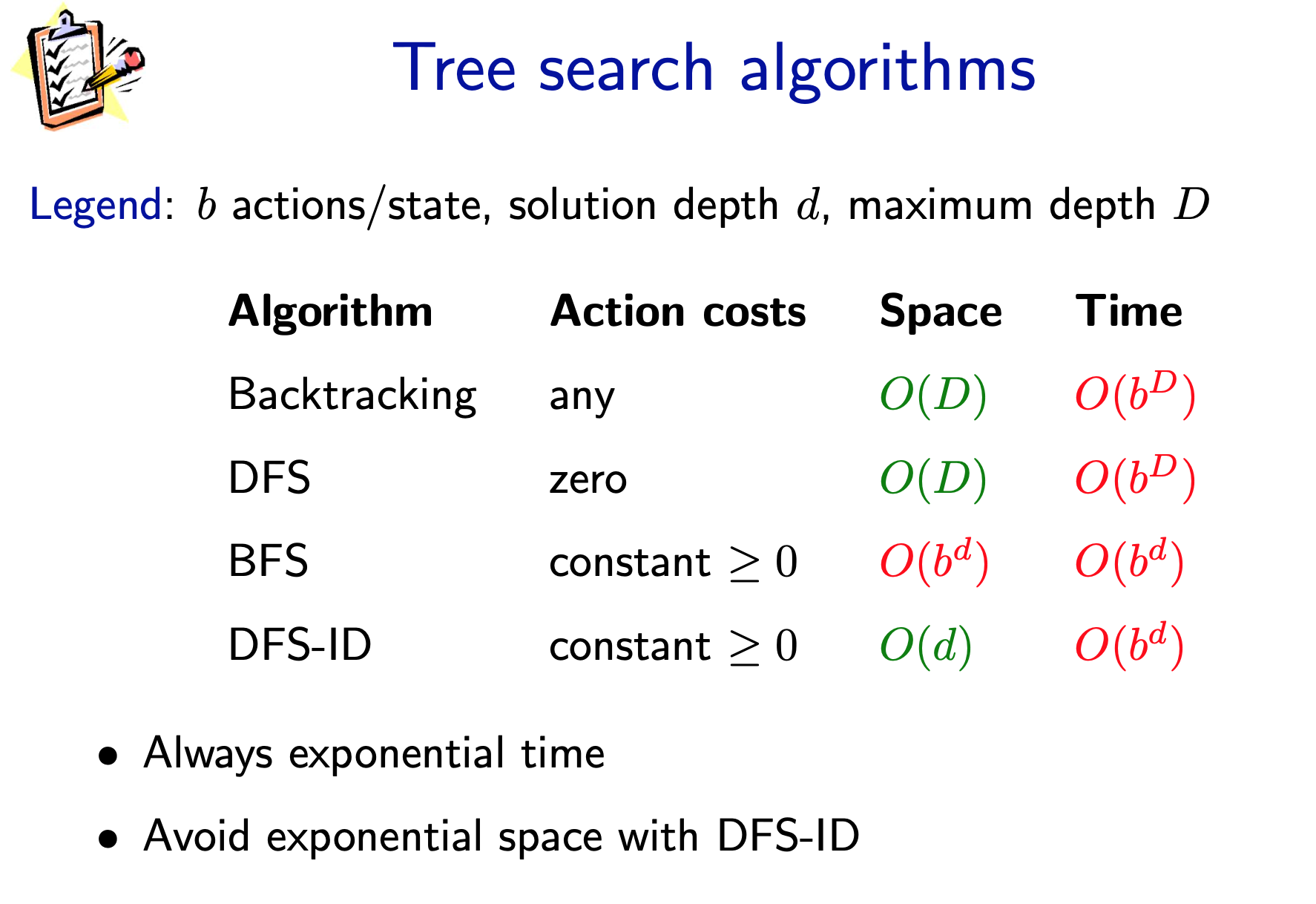
If b actions per state, maximum depth is D actions: - Memory: \(O(D)\) (small) - Time: \(O(b^D)\) (huge) [\(2^{50}\) = 1125899906842624]
We will start with backtracking search, the simplest algorithm which just tries all paths. The algorithm is called recursively on the current state s and the path leading up to that state. If we have reached a goal, then we can update the minimum cost path with the current path. Otherwise, we consider all possible actions a from state s, and recursively search each of the possibilities.
Graphically, backtracking search performs a depth-first traversal of the search tree. What is the time and memory complexity of this algorithm? To get a simple characterization, assume that the search tree has maximum depth D (each path consists of D actions/edges) and that there are b available actions per state (the branching factor is b). It is easy to see that backtracking search only requires O(D) memory (to maintain the stack for the recurrence), which is as good as it gets.
However, the running time is proportional to the number of nodes in the tree, since the algorithm needs to check each of them. The number of nodes is
\[1 + b + b^{2} + \cdots + b^{D} = \frac{b^{D+1} - 1}{B-1} = O(b^{D})\]
Note that the total number of nodes in the search tree is on the same order as the number of leaves, so the cost is always dominated by the last level.
Depth-first search
- Assume action costs Cost(s, a) = 0.
- Idea: Backtracking search + stop when find the first end state.
- If b actions per state, maximum depth is D actions:
- Memory: \(O(D)\) (small)
- Time: \(O(b^D)\) worst case but could be much better if solutions are easy to find.
Backtracking search will always work (i.e., find a minimum cost path), but there are cases where we can do it faster. But in order to do that, we need some additional assumptions — there is no free lunch. Suppose we make the assumption that all the action costs are zero. In other words, all we care about is finding a valid action sequence that reaches the goal. Any such sequence will have the minimum cost: zero.
In this case, we can just modify backtracking search to not keep track of costs and then stop searching as soon as we reach a goal. The resulting algorithm is depth-first search (DFS), which should be familiar to you. The worst time and space complexity are of the same order as backtracking search. In particular, if there is no path to an end state, then we have to search the entire tree.
Breadth-first search
- Assume action costs Cost(s, a) = c for some c >= 0.
- Idea: explore all nodes in order of increasing depth.
- Legend: b actions per state, solution has d actions
- Memory: \(O(b^{d})\) (small)
- Time: \(O(b^d)\) (better, depends on d, not D).
Breadth-first search (BFS), which should also be familiar, makes a less stringent assumption, that all the action costs are the same non-negative number. This effectively means that all the paths of a given length have the same cost. BFS maintains a queue of states to be explored. It pops a state off the queue, then pushes its successors back on the queue.
DFS with iterative deepening
- Assume action costs Cost(s, a) = c for some c ≥ 0.
- Modify DFS to stop at a maximum depth.
- Call DFS for maximum depths 1,2,....
- Memory: \(O(d)\) (sabed!)
- Time: \(O(b^d)\) (same as BFS).
1 | def backtrackingSearch(problem): |
Dynamic programming
backtracking search with memoization — potentially exponential savings
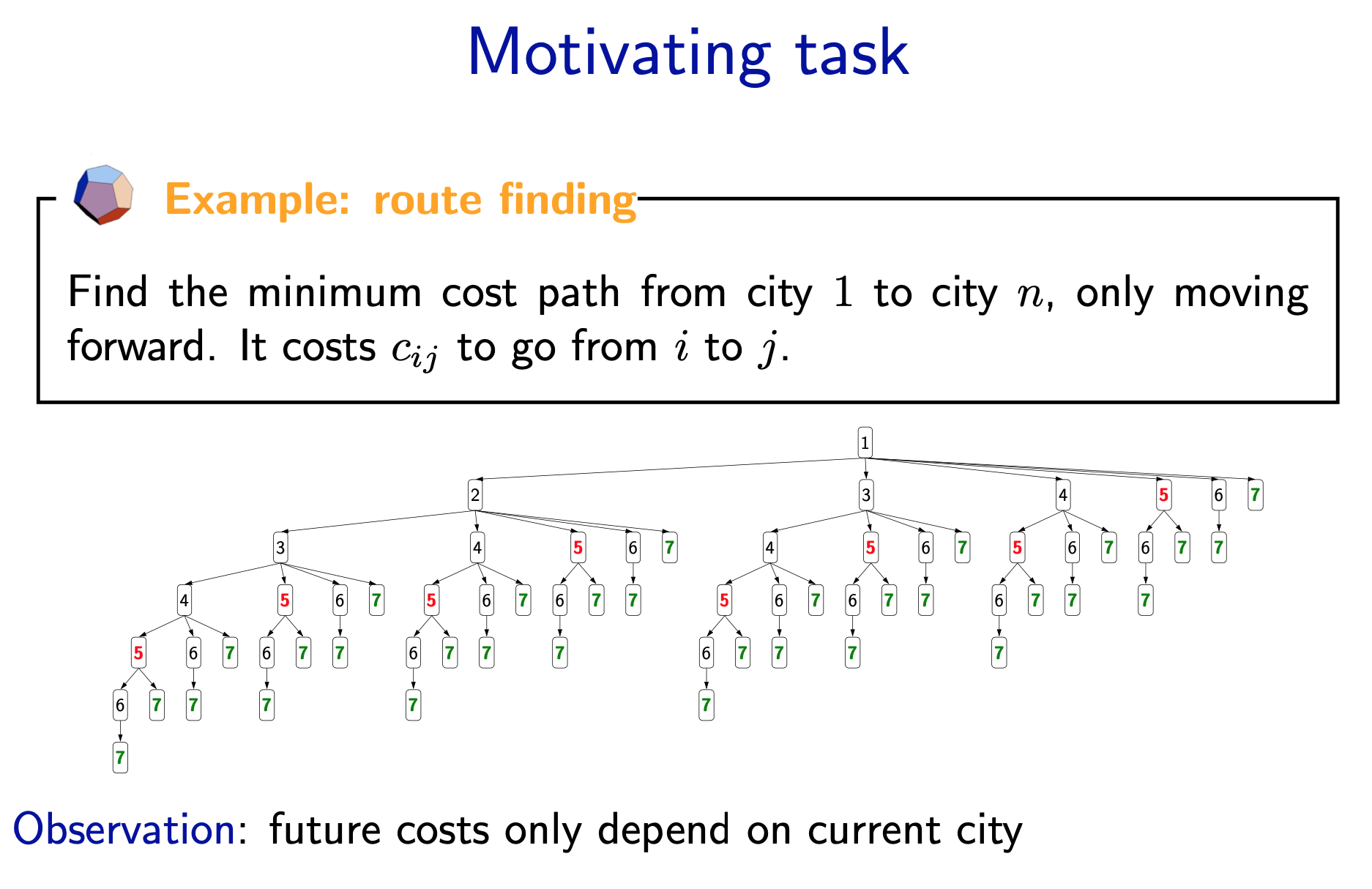
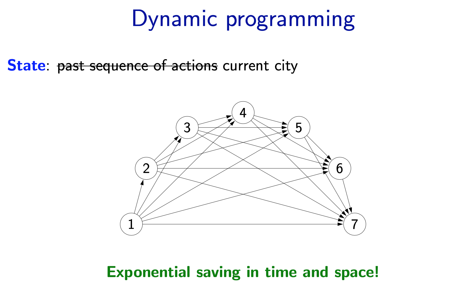
- Now let us see if we can avoid the exponential time. If we consider the simple route finding problem of traveling from city 1 to city n, the search tree grows exponentially with n.
- However, upon closer inspection, we note that this search tree has a lot of repeated structures. Moreover (and this is important), the future costs (the minimum cost of reaching a end state) of a state only depends on the current city! So therefore, all the subtrees rooted at city 5, for example, have the same minimum cost!
- If we can just do that computation once, then we will have saved big time. This is the central idea of dynamic programming.
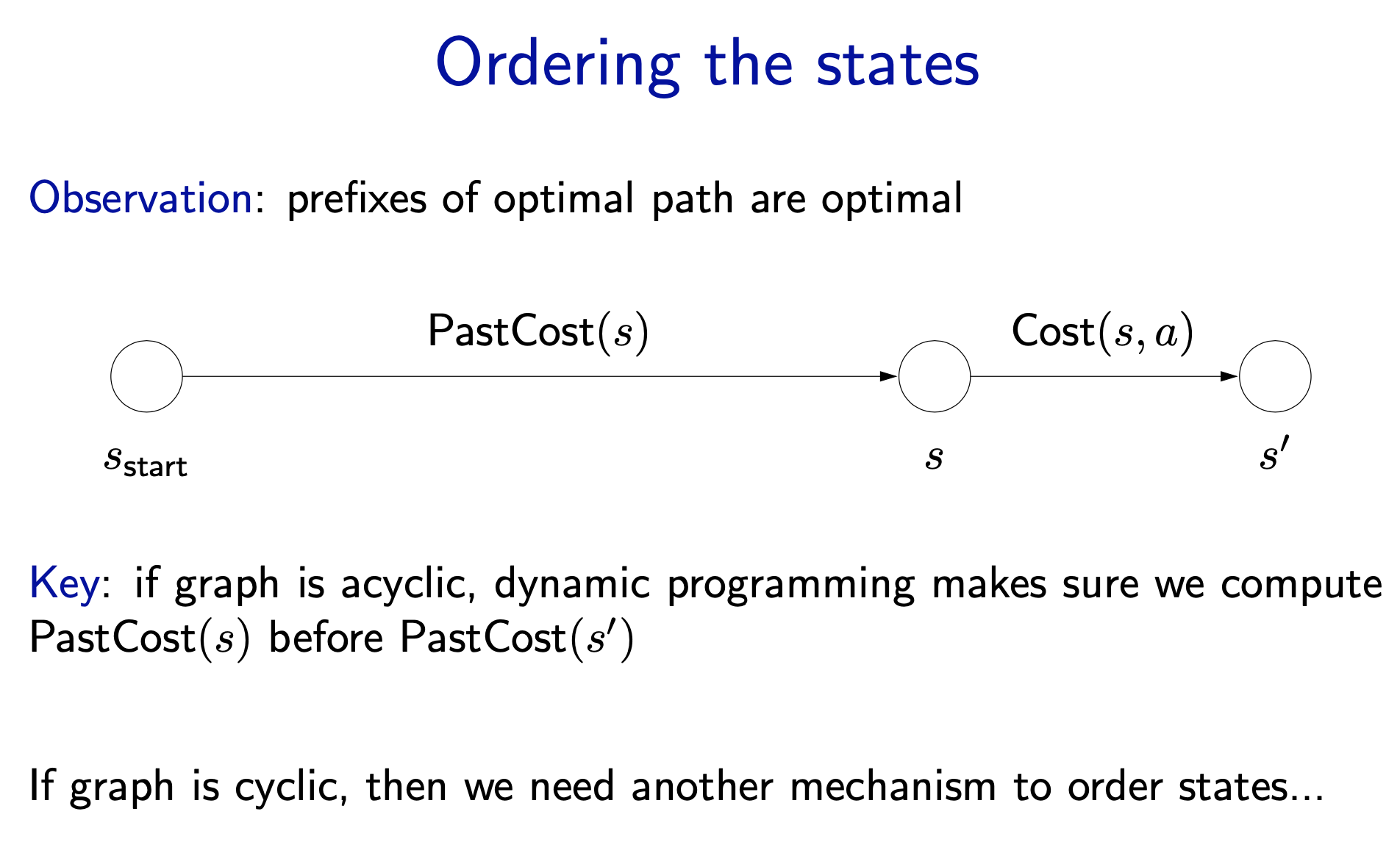
- The dynamic programming algorithm is exactly backtracking search with one twist. At the beginning of the function, we check to see if we’ve already computed the future cost for s. If we have, then we simply return it (which takes constant time if we use a hash map). Otherwise, we compute it and save it in the cache so we don’t have to recompute it again. In this way, for every state, we are only computing its value once.
- One important point is that the graph must be acyclic for dynamic programming to work. If there are cycles, the computation of a future cost for s might depend on \(s^{\prime}\) which might depend on s. We will infinite loop in this case. To deal with cycles, we need uniform cost search, which we will describe later.
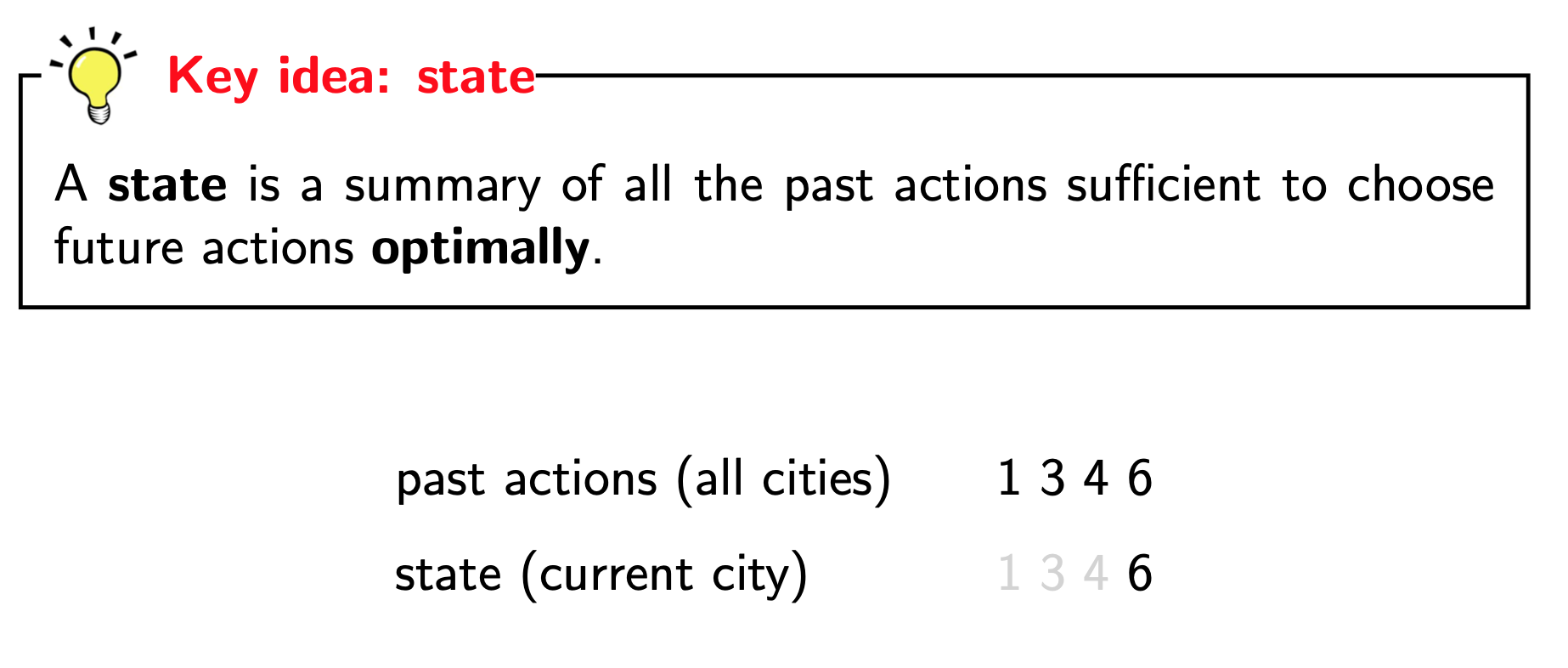
- This is perhaps the most important idea of this lecture: state. A state is a summary of all the past actions sufficient to choose future actions optimally.
- What state is really about is forgetting the past. We can’t forget everything because the action costs in the future might depend on what we did on the past. The more we forget, the fewer states we have, and the more efficient our algorithm. So the name of the game is to find the minimal set of states that suffice. It’s a fun game.
1 | def dynamicProgramming(problem): |
Uniform cost search
- UCS enumerates states in order of increasing past cost.
- All action costs are non-negative: Cost(s, a) ≥ 0.
- The key idea that uniform cost search (UCS) uses is to compute the past costs in order of increasing past cost. To make this efficient, we need to make an important assumption that all action costs are non-negative.
- This assumption is reasonable in many cases, but doesn’t allow us to handle cases where actions have payoff. To handle negative costs (positive payoffs), we need the Bellman-Ford algorithm. When we talk about value iteration for MDPs, we will see a form of this algorithm.
- Note: those of you who have studied algorithms should immediately recognize UCS as Dijkstra’s algorithm. Logically, the two are indeed equivalent. There is an important implementation difference: UCS takes as input a search problem, which implicitly defines a large and even infinite graph, whereas Dijkstra’s algorithm (in the typical exposition) takes as input a fully concrete graph. The implicitness is important in practice because we might be working with an enormous graph (a detailed map of world) but only need to find the path between two close by points (Stanford to Palo Alto).
High-level strategy
- Explored: states we've found the optimal path to
- Frontier: states we've seen, still figuring out how to get there cheaply
- Unexplored: states we haven't seen
The general strategy of UCS is to maintain three sets of nodes: explored, frontier, and unexplored. Throughout the course of the algorithm, we will move states from unexplored to frontier, and from frontier to explored. The key invariant is that we have computed the minimum cost paths to all the nodes in the explored set. So when the end state moves into the explored set, then we are done.
1 | def uniformCostSearch(problem): |
Reference
- CS221 course note and ppt https://stanford-cs221.github.io/autumn2019/