0%

Decision Boundry

Decision Boundry

  1. 决策边界:在特征空间内,根据不同特征对样本进行分类,不同类型间的分界就是模型针对该数据集的决策边界;
  2. 通过决策边界可以直接根据样本在特征空间的位置对该样本的类型进行预测;
  3. 满足决策边界条件的样本点,分为哪一类都可以,但实际应用中很少发生。

两种特征的数据集的决策边界

  1. 拟合的模型为: \[\theta_0 + \theta_1\cdot x_1 + \theta_2\cdot x_2 = 0\] 则该边界是一条直线,因为分类问题中特征空间的坐标轴都表示特征
  2. Decision Boundry 为: \[x_2 = \frac{-\theta_0 - \theta_1 x_1}{\theta_2}\]
  3. 模拟数据集并绘制
    1
    2
    3
    4
    5
    6
    7
    8
    9
    10
    11
    12
    13
    14
    15
    16
    17
    18
    19
    20
    21
    from playML.train_test_split import train_test_split

    X_train, X_test, y_train, y_test = train_test_split(X, y, seed=666)


    from playML.LogisticRegression import LogisticRegression

    log_reg = LogisticRegression()
    log_reg.fit(X_train, y_train)

    # x2()函数:求满足决策边界关系的直线的函数值;
    def x2(x1):
    return (-log_reg.coef_[0] * x1 - log_reg.intercept_) / log_reg.coef_[1]

    x1_plot = np.linspace(4, 8, 1000)
    x2_plot = x2(x1_plot)

    plt.scatter(X[y==0, 0], X[y==0, 1], color='red')
    plt.scatter(X[y==1, 0], X[y==1, 1], color='blue')
    plt.plot(x1_plot, x2_plot)
    plt.show()

不规则的决策边界的绘制方法

  1. 思路:特征空间中分布着无数的点,通过细分,将特征空间分割无数的点,对于每一个点都使用模型对其进行预测分类,将这些预测结果绘制出来,不同颜色的点的边界就是分类的决策边界
  2. 分割方法:将特征空间的坐标轴等分为 n 份(可视化时只显示两种特征),则特征空间被分割为 \(n \codt n\)个点(每个点相当于一个样本),用模型预测这\(x^2\)个点的类型,经预测结果(样本点)显示在特征空间;
1
2
3
4
5
6
7
8
9
10
11
12
13
14
15
16
17
18
19
20
21
22
23
24
25
26
27
28
29
30
31
32
33
34
35
36
# plot_decision_boundary()函数:绘制模型在二维特征空间的决策边界;
def plot_decision_boundary(model, axis):
# model:算法模型;
# axis:区域坐标轴的范围,其中 0,1,2,3 分别对应 x 轴和 y 轴的范围;

# 1)将坐标轴等分为无数的小点,将 x、y 轴分别等分 (坐标轴范围最大值 - 坐标轴范围最小值)*100 份,
# np.meshgrid():
x0, x1 = np.meshgrid(
np.linspace(axis[0], axis[1], int((axis[1]-axis[0])*100)).reshape(-1,1),
np.linspace(axis[2], axis[3], int((axis[3]-axis[2])*100)).reshape(-1,1)
)
# np.c_():
X_new = np.c_[x0.ravel(), x1.ravel()]

# 2)model.predict(X_new):将分割出的所有的点,都使用模型预测
y_predict = model.predict(X_new)
zz = y_predict.reshape(x0.shape)

# 3)绘制预测结果
from matplotlib.colors import ListedColormap
custom_cmap = ListedColormap(['#EF9A9A','#FFF59D','#90CAF9'])

plt.contourf(x0, x1, zz, linewidth=5, cmap=custom_cmap)


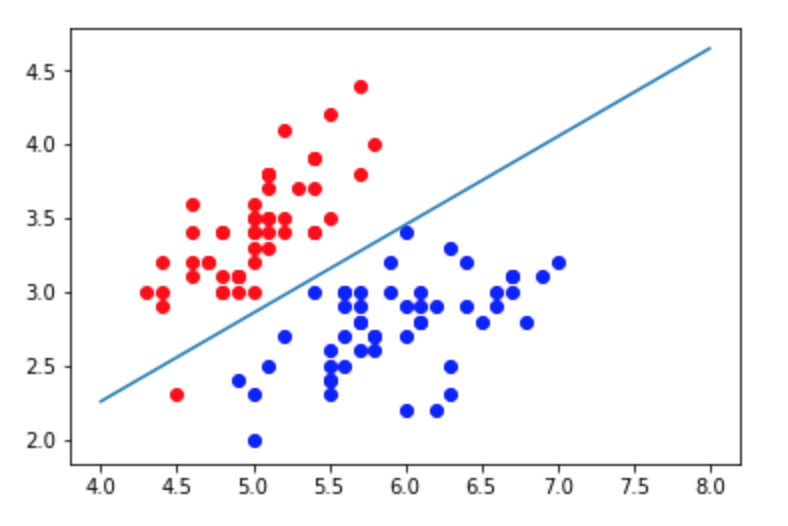
knn_clf_all = KNeighborsClassifier()
knn_clf_all.fit(iris.data[:,:2], iris.target)
# 输出:KNeighborsClassifier(algorithm='auto', leaf_size=30, metric='minkowski',
metric_params=None, n_jobs=1, n_neighbors=5, p=2,
weights='uniform')

plot_decision_boundary(knn_clf_all, axis=[4, 8, 1.5, 4.5])
plt.scatter(iris.data[iris.target==0,0], iris.data[iris.target==0,1])
plt.scatter(iris.data[iris.target==1,0], iris.data[iris.target==1,1])
plt.scatter(iris.data[iris.target==2,0], iris.data[iris.target==2,1])
plt.show()