1
2
3
4
5
6
7
8
9
10
11
12
13
14
15
16
17
18
import numpy as npimport matplotlib.pyplot as pltimport mathfrom sklearn import decompositiondef plot_arrow (ax, start, stop ): ax.annotate('' , xytext=start, xy=stop, arrowprops=dict (facecolor='red' , width=2.0 )) def corr_vars ( start=-10 , stop=10 , step=0.5 , mu=0 , sigma=3 , func=lambda x: x ): x = np.arange(start, stop, step) e = np.random.normal(mu, sigma, x.size) y = np.zeros(x.size) for ind in range (x.size): y[ind] = func(x[ind]) + e[ind] return (x,y)
1 2 3 4 5 6 7 8 9 np.random.seed(100 ) (x1,x2) = corr_vars(start=2 , stop=4 , step=0.2 , sigma=2 , func=lambda x: 2 *math.sin(x)) A = np.column_stack((x1,x2)) Aorig = A A
array([[ 2. , -1.68093609],
[ 2.2 , 2.30235361],
[ 2.4 , 3.65699797],
[ 2.6 , 0.52613067],
[ 2.8 , 2.63261787],
[ 3. , 1.3106777 ],
[ 3.2 , 0.32561105],
[ 3.4 , -2.65116887],
[ 3.6 , -1.26403255],
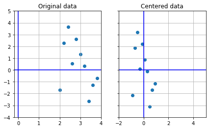
[ 3.8 , -0.71371289]])1 2 3 4 5 6 7 8 9 10 11 12 13 14 15 16 17 18 19 20 A = (A-np.mean(A,axis=0 )) f, (ax1, ax2) = plt.subplots(1 , 2 , sharey=True , figsize=(7 ,4 )) ax1.scatter(Aorig[:,0 ], Aorig[:,1 ]) ax1.set_title("Original data" ) ax1.grid(True ) ax2.scatter(A[:,0 ],A[:,1 ]) ax2.set_title("Centered data" ) ax2.grid(True ) ax1.axhline(0 , color="blue" ) ax1.axvline(0 , color="blue" ) ax2.axhline(0 , color="blue" ) ax2.axvline(0 , color="blue" ) plt.xlim([-2 ,5 ]) plt.ylim([-4 ,5 ])
(-4, 5)
png
1
2
3
4
S = np.dot(A.T,A)/(A.shape[0 ]-1 ) print ("The covariance matrix is:" )print (S,"\n" )
The covariance matrix is:
[[ 0.36666667 -0.55248919]
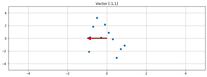
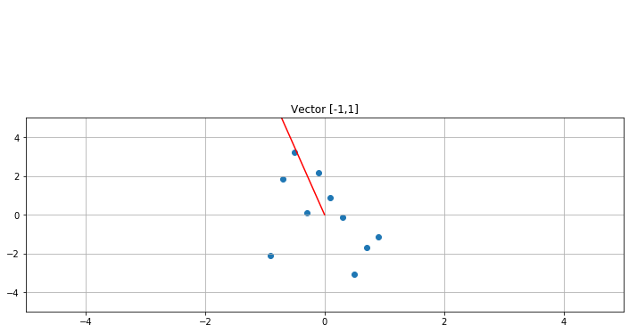
[-0.55248919 4.18798554]] 1 2 3 4 5 6 7 8 9 10 11 f, ax1 = plt.subplots(1 , 1 , sharey=True , figsize=(12 ,4 )) V = np.array([[-1 ],[0 ]]) print ("Vector slope: " ,V[1 ]/V[0 ])ax1.scatter(A[:,0 ],A[:,1 ]) ax1.set_title("Vector [-1,1]" ) ax1.grid(True ) ax1.plot([0 ,V[0 ]],[0 ,V[1 ]],c='r' ) plot_arrow(ax1, (0 ,0 ),(V[0 ],V[1 ])) plt.xlim([-5 ,5 ]) plt.ylim([-5 ,5 ])
Vector slope: [-0.]
(-5, 5)
png
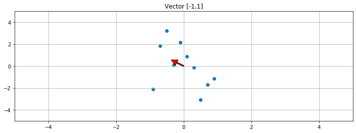
1 2 3 4 5 6 7 8 9 10 11 12 f, ax1 = plt.subplots(1 , 1 , sharey=True , figsize=(12 ,4 )) V = np.dot(S,V) print ("Vector slope: " ,V[1 ]/V[0 ])ax1.scatter(A[:,0 ],A[:,1 ]) ax1.set_title("Vector [-1,1]" ) ax1.grid(True ) ax1.plot([0 ,V[0 ]],[0 ,V[1 ]],c='r' ) plot_arrow(ax1, (0 ,0 ),(V[0 ],V[1 ])) plt.xlim([-5 ,5 ]) plt.ylim([-5 ,5 ])
Vector slope: [-1.50678871]
(-5, 5)
png
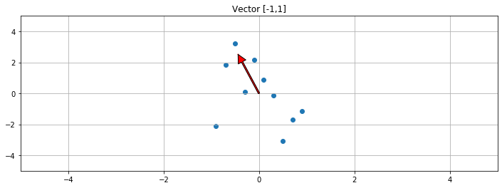
1
2
3
4
5
6
7
8
9
10
11
12
f, ax1 = plt.subplots(1 , 1 , sharey=True , figsize=(12 ,4 )) V = np.dot(S,V) print ("Vector slope: " ,V[1 ]/V[0 ])ax1.scatter(A[:,0 ],A[:,1 ]) ax1.set_title("Vector [-1,1]" ) ax1.grid(True ) ax1.plot([0 ,V[0 ]],[0 ,V[1 ]],c='r' ) plot_arrow(ax1, (0 ,0 ),(V[0 ],V[1 ])) plt.xlim([-5 ,5 ]) plt.ylim([-5 ,5 ])
Vector slope: [-5.72313052]
(-5, 5)
png
1
2
3
4
5
6
7
8
9
10
11
12
f, ax1 = plt.subplots(1 , 1 , sharey=True , figsize=(12 ,4 )) V = np.dot(S,V) print ("Vector slope: " ,V[1 ]/V[0 ])ax1.scatter(A[:,0 ],A[:,1 ]) ax1.set_title("Vector [-1,1]" ) ax1.grid(True ) ax1.plot([0 ,V[0 ]],[0 ,V[1 ]],c='r' ) plot_arrow(ax1, (0 ,0 ),(V[0 ],V[1 ])) plt.xlim([-5 ,5 ]) plt.ylim([-5 ,5 ])
Vector slope: [-6.94911232]
(-5, 5)
png
1 2 3 4 5 6 7 8 9 10 11 12 13 14 print ("The slope of the vector converges to the direction of greatest variance:\n" )V = np.dot(S,V) print ("Vector slope: " ,V[1 ]/V[0 ])V = np.dot(S,V) print ("Vector slope: " ,V[1 ]/V[0 ])V = np.dot(S,V) print ("Vector slope: " ,V[1 ]/V[0 ])V = np.dot(S,V) print ("Vector slope: " ,V[1 ]/V[0 ])V = np.dot(S,V) print ("Vector slope: " ,V[1 ]/V[0 ])V = np.dot(S,V) print ("Vector slope: " ,V[1 ]/V[0 ])
The slope of the vector converges to the direction of greatest variance:

Vector slope:  [-7.0507464]
Vector slope:  [-7.0577219]
Vector slope:  [-7.05819391]
Vector slope:  [-7.05822582]
Vector slope:  [-7.05822798]
Vector slope:  [-7.05822813]
1 2 3 4 5 6 7 8 l_1 = (S.trace() + np.sqrt(pow (S.trace(),2 ) - 4 *np.linalg.det(S))) / 2 l_2 = (S.trace() - np.sqrt(pow (S.trace(),2 ) - 4 *np.linalg.det(S))) / 2 print ("The eigenvalues are:" )print ("L1:" ,l_1)print ("L2:" ,l_2)
The eigenvalues are:
L1: 4.266261447240239
L2: 0.28839076171131417
1 2 3 4 5 6 7 8 9 10 11 12 13 14 15 A1 = S - l_1 * np.identity(2 ) A2 = S - l_2 * np.identity(2 ) E1 = A2[:,1 ] E2 = A1[:,0 ] E1 = E1 / np.linalg.norm(E1) E2 = E2 / np.linalg.norm(E2) print ("The eigenvectors are:" )print ("E1:" , E1)print ("E2:" , E2)
The eigenvectors are:
E1: [-0.14027773  0.9901122 ]
E2: [-0.9901122  -0.14027773]
1 2 3 E = np.column_stack((E1,E2)) E
array([[-0.14027773, -0.9901122 ],
[ 0.9901122 , -0.14027773]])1 2 3 4 evals, evecs = np.linalg.eigh(S) print (evals)print (evecs)
[0.28839076 4.26626145]
[[-0.9901122 -0.14027773]
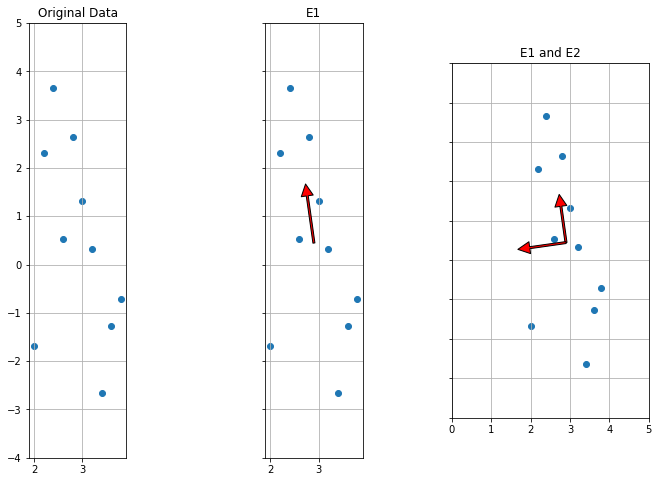
[-0.14027773 0.9901122 ]]1 2 3 4 5 6 7 8 9 10 11 12 13 14 15 16 17 18 19 20 21 f, (ax1, ax2, ax3) = plt.subplots(1 , 3 , sharey=True , figsize=(12 ,8 )) ax1.scatter(Aorig[:,0 ],Aorig[:,1 ]) ax1.set_title("Original Data" ) ax1.grid(True ) ax1.set_aspect('equal' ) ax2.scatter(Aorig[:,0 ],Aorig[:,1 ]) ax2.set_title("E1" ) ax2.grid(True ) plot_arrow(ax2, np.mean(Aorig,axis=0 ), np.mean(Aorig,axis=0 ) + np.dot(Aorig, E).std(axis=0 ).mean() * E1) ax2.set_aspect('equal' ) ax3.scatter(Aorig[:,0 ],Aorig[:,1 ]) ax3.set_title("E1 and E2" ) ax3.grid(True ) plot_arrow(ax3, np.mean(Aorig,axis=0 ), np.mean(Aorig,axis=0 ) + np.dot(Aorig, E).std(axis=0 ).mean() * E1) plot_arrow(ax3, np.mean(Aorig,axis=0 ), np.mean(Aorig,axis=0 ) + np.dot(Aorig, E).std(axis=0 ).mean() * E2) ax3.set_aspect('equal' ) plt.xlim([0 ,5 ]) plt.ylim([-4 ,5 ])
(-4, 5)
png
1 2 3 4 5 F1 = np.dot(A, E1) F2 = np.dot(A, E2) F = np.column_stack((F1, F2)) F
array([[-1.97812455,  1.18924584],
       [ 1.93772363,  0.43245658],
       [ 3.25091797,  0.04440771],
       [ 0.12295254,  0.28557622],
       [ 2.18055566, -0.20793946],
       [ 0.84363103, -0.22052313],
       [-0.15975102, -0.28036266],
       [-3.13515266, -0.06080918],
       [-1.78978762, -0.45341595],
       [-1.27296497, -0.72863598]])
1 2 pca = decomposition.PCA(n_components=2 ) print (pca.fit_transform(A))
[[-1.97812455  1.18924584]
 [ 1.93772363  0.43245658]
 [ 3.25091797  0.04440771]
 [ 0.12295254  0.28557622]
 [ 2.18055566 -0.20793946]
 [ 0.84363103 -0.22052313]
 [-0.15975102 -0.28036266]
 [-3.13515266 -0.06080918]
 [-1.78978762 -0.45341595]
 [-1.27296497 -0.72863598]]