Adversarial Autoencoders

Category: Article
Created: January 25, 2022 4:01 PM
Status: Open
URL: https://arxiv.org/abs/1511.05644
Updated: January 29, 2022 11:39 AM

Highlights

We propose a general approach, called an adversarial autoencoder (AAE) that can turn an autoencoder into a generative model.
An autoencoder is trained with dual objectives – a traditional reconstruction error criterion, and an adversarial training criterion.

Methods

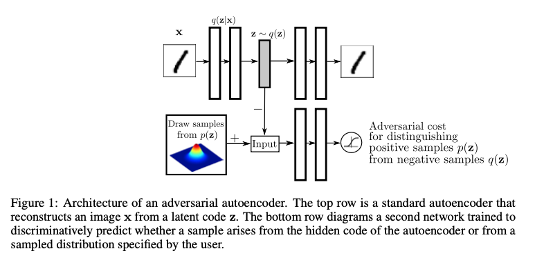
The adversarial autoencoder is an autoencoder that is regularized by matching the aggregated posterior, \(q(z)\), to an arbitrary prior, \(p(z)\). In order to do so, an adversarial network is attached on top of the hidden code vector of the autoencoder as illustrated in Figure 1. It is the adversarial network that guides \(q(z)\) to match \(p(z)\). The autoencoder, meanwhile, attempts to minimize the reconstruction error. The generator of the adversarial network is also the encoder of the autoencoder \(q(z|x)\). The encoder ensures the aggregated posterior distribution can fool the discriminative adversarial network into thinking that the hidden code \(q(z)\) comes from the true prior distribution \(p(z)\).

Training

Both, the adversarial network and the autoencoder are trained jointly with SGD in two phases – the reconstruction phase and the regularization phase – executed on each mini-batch. In the reconstruction phase, the autoencoder updates the encoder and the decoder to minimize the reconstruction error of the inputs. In the regularization phase, the adversarial network first updates its discriminative network to tell apart the true samples (generated using the prior) from the generated samples (the hidden codes computed by the autoencoder). The adversarial network then updates its generator (which is also the encoder of the autoencoder) to confuse the discriminative network.

Incorporating Label Information in the Adversarial Regularization

In the scenarios where data is labeled, we can incorporate the label information in the adversarial training stage to better shape the distribution of the hidden code.

We now aim to force each mode of the mixture of Gaussian distribution to represent a single label of MNIST.

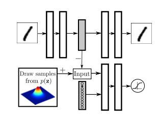
Regularizing the hidden code by providing a one-hot vector to the discriminative network. The one-hot vector has an extra label for training points with unknown classes.

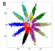
B is valina AAE.
A is AAE incorporated with label information

Supervised Adversarial Autoencoders

In order to incorporate the label information, we alter the network architecture to provide a one-hot vector encoding of the label to the decoder. The decoder utilizes both the one-hot vector identifying the label and the hidden code \(z\) to reconstruct the image. This architecture forces the network to retain all information independent of the label in the hidden code \(z\).

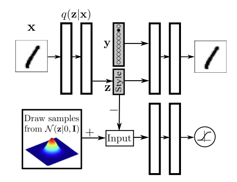
Disentangling the label information from the hidden code by providing the one-hot vector to the generative model. The hidden code in this case learns to represent the style of the image.

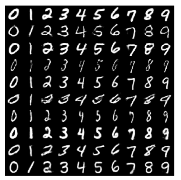
Each row presents reconstructed images in which the hidden code z is fixed to a particular value but the label is systematically explored.

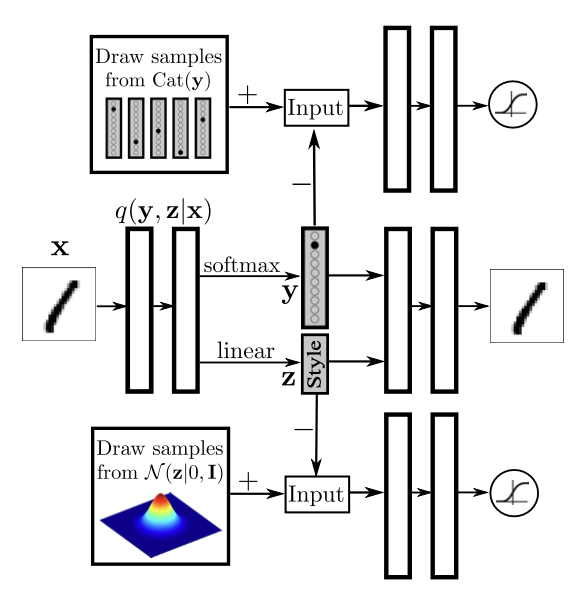
Semi-Supervised Adversarial Autoencoders

we now use the adversarial autoencoder to develop models for semi-supervised learning that exploit the generative description of the unlabeled data to improve the classification performance that would be obtained by using only the labeled data.
we assume the data is generated by a latent class variable y that comes from a Categorical distribution as well as a continuous latent variable z that comes from a Gaussian distribution:

\(p(y) = Cat(y)\)

\(p(z) = N(z | 0, I)\)
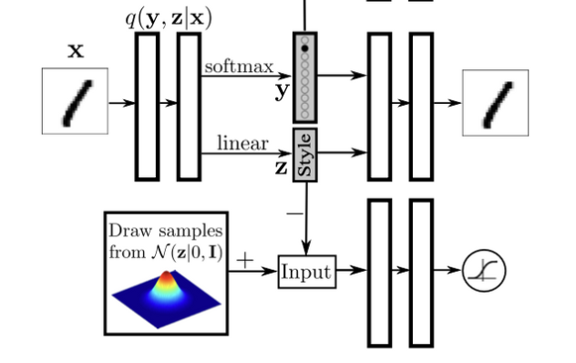
Semi-Supervised AAE: the top adversarial network imposes a Categorical distribution on the label representation and the bottom adversarial network imposes a Gaussian distribution on the style representation. \(q(y|x)\) is trained on the labeled data in the semi-supervised settings.

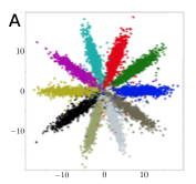
Unsupervised Clustering with Adversarial Autoencoders

the adversarial autoencoder can disentangle discrete class variables from the continuous latent style variables in a purely unsupervised fashion.
with the difference that we remove the semi- supervised classification stage and thus no longer train the network on any labeled mini-batch.
Another difference is that the inference network \(q(y|x)\) predicts a one-hot vector whose dimension is the number of categories that we wish the data to be clustered into.

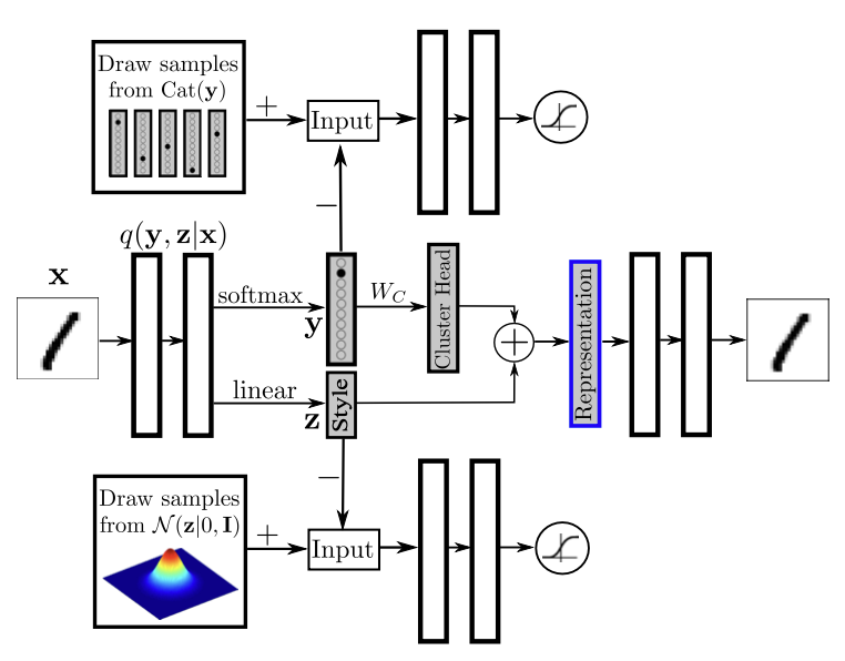
Dimensionality Reduction with Adversarial Autoencoders

Dimensionality reduction with adversarial autoencoders: There are two separate adversarial networks that impose Categorical and Gaussian distribution on the latent representation. The final \(n\) dimensional representation is constructed by first mapping the one-hot label representation to an \(n\) dimensional cluster head representation and then adding the result to an n dimensional style representation. ****