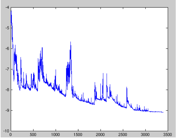
An overview of gradient descent optimization algorithms

Reference from An overview of gradient descent optimization algorithms

Batch gradient descent

\[\theta = \theta - \eta * \triangledown_{\theta}J(\theta)\]

1
2
3

for i in range(nb_epochs):
  params_grad = evaluate_gradient(loss_function, data, params)
  params = params - learning_rate * params_grad

Batch gradient descent is guaranteed to converge to the global minimum for convex error surfaces and to a local minimum for non-convex surfaces.

Stochastic gradient descent

\[\theta = \theta - \eta * \triangledown_{\theta}J(\theta; x^{i};y^{i})\]

for i in range(nb_epochs):
  np.random.shuffle(data)
  for example in data:
    params_grad = evaluate_gradient(loss_function, example, params)
    params = params - learning_rate * params_grad

SGD performs frequent updates with a high variance that cause the objective function to fluctuate heavily as in Image 1.
SGD shows the same convergence behaviour as batch gradient descent, almost certainly converging to a local or the global minimum for non-convex and convex optimization respectively.

Mini-batch gradient descent

\[\theta = \theta - \eta * \triangledown_{\theta}J(\theta; x^{i:i+n};y^{i:i+n})\]

for i in range(nb_epochs):
  np.random.shuffle(data)
  for batch in get_batches(data, batch_size=50):
    params_grad = evaluate_gradient(loss_function, batch, params)
    params = params - learning_rate * params_grad

Common mini-batch sizes range between 50 and 256, but can vary for different applications
Mini-batch gradient descent is typically the algorithm of choice when training a neural network and the term SGD usually is employed also when mini-batches are used

Challenges

Choosing a proper learning rate can be difficult
the same learning rate applies to all parameter updates
Learning rate schedules
- ry to adjust the learning rate during training by e.g. annealing
- reducing the learning rate according to a pre-defined schedule or when the change in objective between epochs falls below a threshold
Another key challenge of minimizing highly non-convex error functions common for neural networks is avoiding getting trapped in their numerous suboptimal local minima

Momentum

Momentum is a method that helps accelerate SGD in the relevant direction and dampens oscillations as can be seen in Image 3. It does this by adding a fraction of the update vector of the past time step to the current update vector:

\[ \begin{align*} & v_{t} = \gamma v_{t-1} + \eta * \triangledown_{\theta}J(\theta) \\ & \theta = \theta - v_{t}\\ \end{align*} \]

The momentum term \(\gamma\) is usually set to 0.9 or a similar value.
The ball accumulates momentum as it rolls downhill, becoming faster and faster on the way

Nesterov accelerated gradient

\[ \begin{align*} & v_{t} = \gamma v_{t-1} + \eta * \triangledown_{\theta}J(\theta - \gamma * m) \\ & \theta = \theta - v_{t}\\ \end{align*} \]

既然参数要沿着 \(\theta - \gamma * m\)更新，那就先先计算未来位置的梯度
This anticipatory update prevents us from going too fast and results in increased responsiveness, which has significantly increased the performance of RNNs on a number of tasks

Adagrad

\[ \begin{align*} & s = s + \triangledown J(\theta) \bigodot \triangledown J(\theta) \\ & \theta = \theta - \frac{\eta}{\sqrt{s + \epsilon}} \bigodot \triangledown J(\theta) \\ \end{align*} \]

One of Adagrad's main benefits is that it eliminates the need to manually tune the learning rate
Adagrad modifies the general learning rate \(\gamma\) at each time step t for every parameter \(\theta_{i}\) based on the past gradients that have been computed for \(\theta_{i}\)

RMSprop

\[ \begin{align*} & v_{t} = \gamma v_{t-1} + (1-\gamma) * \triangledown J(\theta) \bigodot \triangledown J(\theta) \\ & \theta = \theta - v_{t} \\ \end{align*} \]

1	tf.train.RMSPropOptimizer(learning_rate=learning_rate, momentum=0.9, decay=0.9, epsilon=1e-10)

加入Momentum，主要是解决学习速率过快衰减的问题
RMSprop as well divides the learning rate by an exponentially decaying average of squared gradients. Hinton suggests \(\gamma\) to be set to 0.9, while a good default value for the learning rate \(\eta\) is 0.001.

Adaptive moment estimation (Adam)

\[ \begin{align*} & m = \beta_{1} * m + (1-\beta_{1}) * \triangledown J(\theta) \\ & s = \beta_{2} * s + (1-\beta_{2}) * \triangledown J(\theta) \bigodot \triangledown J(\theta) \\ & m = \frac{m}{1-\beta^{t}_{1}} \\ & s = \frac{s}{1-\beta^{t}_{2}} \\ & \theta = \theta - \frac{\eta}{\sqrt{s + \epsilon}} \bigodot m \end{align*} \]

其结合了Momentum和RMSprop算法的思想。相比Momentum算法，其学习速率是自适应的，而相比RMSprop，其增加了冲量项, 第三和第四项主要是为了放大它们
The authors propose default values of 0.9 for \(\beta1\), 0.9999 for \(\beta2\) and \(10^{-8}\) for \(\epsilon\)